Adam Ginsburg's blog

• Spatial Transfer Functions

  The majority of the past week has been dedicated to debugging; it looks like cross-scanned simulations finally work. The plot below is a derivation of the spatial transfer function for a number of different intrinsic sky power-law power spectra.

  

  Justifying the above plot is essential. First, the very steep power-laws [-3 in the example below] show a recovery fraction >1. This is simply because their S/N was inadequate - the output power spectrum is nearly flat, but at a level higher than the sky.

  

  Second, the most plausible power-laws [-1.5 in the example below] show pretty good recovery (90-95% over the relevant range):

  

  There are some "white" power losses, particularly in the flatter power-spectra. My best guess is that this has something to do with the relative scales being offset from a mean of 1, but so far all tests to show that that is the cause have in fact shown no problems at all. What else could cause a scale-independent power loss? Also, the flat power spectrum (and inverted) aren't quite flat because I impose a "galactic scale height" on them. Should I stop doing that?

---

• Measuring preferred angles in the Herschel data on larger scales

  This is something of a repeat of yesterday's exercise, but for Herschel data on larger scales, where filamentation is expected (at different angles?) on a different scale than the Galactic plane. First example: L030 500 microns

  

  There is evidently a preferred direction that is correlated down to the resolution of the map, though the preference is smallest at the smallest scales. This may simply be a statement that there are more sources along the galactic plane, though, since there really isn't any particularly obvious filamentation in the image.

  

  In L59, on the other hand, there is at most a very weak preference except at the largest scales corresponding to the Galactic Plane. This is somewhat interesting because there IS obvious filamentation in the L59 image, but it does not have a preferred direction. Unfortunately, it is not obvious whether or where filamentation shows up in fourier space if it does not have a preferred direction. There is no excess at any spatial scale that I can pick out.

---

• Hunting for preferred directions

  In our last group meeting, we discussed simulations using filamentary structures. I've been trying to determine how best to generate random/artificial filamentary structures in images. The first step in that direction is coming up with a way to measure asymmetries and therefore preferred directions within a real map. In order to do this, I've had to develop a number of new tools in agpy for azimuthally binned radial profiles and radially-averaged azimuthal profiles (radialprofile.py). Examining real maps is necessary because a simple sinusoidal dependence of the power introduces filamentation along the same directions at ALL scales, which is not obviously (or in some cases, obviously not) the correct solution. Filaments are observed on large scales, but sometimes there can be 'kinks' in opposite directions on small scales. So, the map I picked to examine was one with the most flagrantly obvious filamentary structure in it: the Motte DR 21 MAMBO map. It was also a choice of convenience because I already had the data on my laptop....

  

  The preferred direction is quite obvious in this map: there is a long filament going up and down the map. Therefore, the DC component should be substantially higher in one direction than the other.

  

  In the power-spectral-density image, it is quite clear that there is a preferred direction, though it is not obvious that the fourier transform is rotated 90 degrees from the image. My fourier intuition somewhat fails me here.... I realize that a broad, smooth profile in real space should be narrow and highly peaked in fourier space, but I don't fully understand why it effectively spreads out in the perpendicular direction, which I have confirmed that it does with a simple experiment. I also don't know what the Shah function is, but it implies a periodic dip in the image at every 1/5th of the image, or every 50 pixels.

  

  These are the power spectra averaged over different angles as labeled. -15 corresponds to -15 to +15, 15 corresponds to 15 to 45, etc. The highly peaked 75-105 power spectrum shows the large-scale filamentary profile. I think the difference in the DC component is actually an artifact of the azimuthal binning process: each pixel can only be assigned one angle, so the DC value isn't included in all of them... I'll need to find a workaround for that because it's quite deceptive.

  

  The more interesting way to view the data - and perhaps to analyze maps - is to take radial averages in some range of spatial scales and plot the azimuthal dependence. There is a clear sinusoid at large scales. The legend shows "spatial frequency" in 1/pixel units. The distribution becomes more even with angle and even changes preferred direction at smaller scales (higher frequencies). Next step is testing different approaches. I think an added, steeper-power-law component would probably be the best way to start. Another suggestion, courtesy Bruce Elmegreen, is to attempt this sort of asymmetric power law sampling in 3 dimensions (with only 1 or 2 dimensions asymmetric) and then projecting down onto two dimensions.

---

• Recovery as a function of bolometer noise part 2

  In the Experiment 7 simulations I was running, I observed greater noise than expected, causing me to question the results of the previous post. I therefore ran Experiment 8, which is the same as Experiment 6 from that post with a larger (320x320) map with a larger step size. The noise recovery remains linear, but the scaling is quite different - a factor of ~4 instead of ~12. The step size is the most likely culprit, since an 8x larger step size should result in sqrt(8)~2.8 worse noise per pixel.

  

  There are some curious / worrisome artifacts that turn up and are evident in the recovery fraction plot. For the low-noise cases, the middle bolometers get totally flagged out because they are over-weighted (by orders of magnitude).

  

  So I'm forced to explore via pyflagger. I will almost certainly need to re-run all experiments after making a change to how weights are computed. Well, it turns out the problem is that those 28 bolos are scaled to zero, even though there is nothing obvious (or even suggestive) in their timestream plots. This is only true when varyrelscale is off. Apparently varying the relative scales leads to a different problem. AHA! The noise is so low that the relative scales are SO well correlated that the signal is enough to cause problems! A plausible solution is therefore no change to the pipeline, but to add minimal (nominal) noise to the relative scales to increase the MAD so that the others don't get flagged out. So I added a 1% variation, which prevented flagging at the scale stage, but there are still some disturbing artifacts in the map:

  

  Unfortunately, this problem requires further examination in detail. Exp 9/10 should probably be gaussians and airys on larger step-size maps, but the solution will require something else, possibly even a change in the pipeline. On the plus side, I think I can re-run experiment 7 with a factor of 4 instead of 12 scaling for the noise and expect it to work.

---

• Recovery as a function of bolometer noise

  One clear simulation result comes from varying the amplitude of the gaussian noise added to each bolometer's timestream for a fixed atmosphere amplitude. The atmosphere amplitude sets the mean value of the atmosphere timestream. Increased bolometer noise results in decreased recovery of the outer rings of the PSF. This is demonstrated in that the peak amplitudes remain constant (as long as they are still recovered) while the aperture sums (in 100" radius apertures) decrease. The simulations were run on a logarithmic spacing from 1e-3 to 1e0. The 1e0 point is missing because the peak flux wasn't recovered by the gaussian fitter. The model maps don't recover the source at all for this run, which is worrisome, since it means there is no iterative process There is a minor concern that some simulations over-recover the peak at high noise, but the effect is at a <1% level so not very worrisome.

  

  From the same set of simulations, I derive the pixel RMS of the map (the noise level) derived from a give individual bolometer noise. The theoretical expectation would be Measured Noise = Input Noise / N(bolometers) if the pixel sampling and the timestream sampling were the same (i.e. there were exactly sqrt(nbolos) hits per pixel). This is not exactly the case, and there are potential additional sources of noise. Nonetheless, the naive theory appears to be good enough in this simulation:

  

  You can ignore the green/blue points in this plot; they just show that the std. dev. around the source is dominated by the source. Additionally, there is a noise floor, probably set by an inability to model the point source when the S/N gets to be ~500, preventing convergence of the iterator at a level better than 0.2%. In short, though, I'm going to use 1/sqrt(nbolos) to determine the appropriate input noise level in the astro simulations.

---

• Astrophysical Signal Modeling

  Here we finally get into the meat of the simulations. The goal is to develop realistic - but arbitrary - astrophysical models to run through simulations. The first step is to figure out what a realistic sky looks like. To this end, I use the HiGal SDP fields, looking only at their power spectra. They are well represented by a power law with α = 3 (shown in the dashed black line below).

  

  Therefore, I've attempted to randomly sample from a similar power law distribution using the following IDL code:

  dimsize = 512    realpower = realpowers[ii]    imagpower = imagpowers[ii]    imagscale = imagscales[ii]    peakamp = 1.0    noise = 0.03    smoothscale = 2.0    smoothkernel = psf_gaussian(npix=512,ndim=2,fwhm=31.2/7.2/2.0,/normalize)    sigma_gp = 128.0 ; sigma-width of the Galactic Plane (can get more accurate value from Cara's paper)    xx = findgen(dimsize) #  replicate(1.0,dimsize)    yy = findgen(dimsize) ## replicate(1.0,dimsize)    rr = sqrt( (xx-255.5)^2 + (yy-255.5)^2 )    realpart = (rr^realpower) * randomn(seed1,[dimsize,dimsize])    imagpart = ((rr*imagscale)^imagpower) * randomn(seed2,[dimsize,dimsize])*complex(0,1)     fakesky = abs(fft(shift(realpart + imagpart,0,0),1))    expweight = exp(-(yy-255.5)^2/(2.0*sigma_gp^2)) ; most power is in the inner plane    fakesky *= peakamp/max(fakesky)    fakesky_sm = convolve(fakesky,smoothkernel)    fakesky_sm = fakesky_sm*expweight    fakesky_sm += randomn(seed3,[dimsize,dimsize]) * noise

  Since Power is the fourier-transform squared, I'm using a power-law of α=1.5 for the "real" part of the sampling. The imaginary part follows a shallower slope to reduce the amount of power in large structures, which didn't look quite right (but maybe I should leave both slopes the same?). With both the same, and without the imaginary part down-scaled, the structure appears too "cloudy" and not "clumpy" enough. But back to that later...

  The peak amplitude is set by re-scaling the map. Ideally, we'd like to see this set by a point source, since that is true in most fields. The noise level should not be included in simulations, but should be used to show the difference between pipeline-leftover noise and gaussian noise on the sky. i.e., what structures disappear when you just add noise, and what structures are removed by the pipeline.

  The PSF is simply to smooth out signals that are removed by the telescope beam. We can replace this with a "real" PSF if and when we've come up with a believable one.

  The noise is added after the smoothing because it should be on a pixel scale rather than a beam scale.

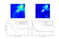
  Here are some example realizations with different power laws:

  

---

• PSF modeling

  There haven't been many posts recently because I've primarily been writing up old results into the v2 paper. The Airy and Gaussian simulations with and without atmosphere seem to have yielded their results. There is a ~5% loss when mapping Airy-disk point sources. This is fine as long as it's quantified; it just means that when calibrating we need to know whether extended sources are similarly truncated. If all sources lose 5% in the pipeline, there will be no net offset. However, the Airy is not necessarily representative of the CSO's PSF. In order to come up with a more reasonable representation of the PSF, I've attempted to fit the *measured* PSF (from James' paper) with an Airy disk. The first sidelobe has a lot more amplitude and is closer to the peak than in an Airy disk. It is also asymmetric, but I'm ignoring that for the moment. To better represent the first sidelobe, I've fitted a modified Airy function. The "modification" is to fit two Airy functions, one to the peak and one to the rest. This is accomplished by setting everything outside the first null to zero in the first function, and everything inside the first null to zero in the second. The centers are the same, but the amplitudes and widths are independent.

  

  The above image shows the best fit Airy and modified Airy, both in log scale on an identical grid. The modeled PSF was then put through the pipeline to see it recovers the pipeline-derived PSF. The radial profile results are below, but note that this is only one particular realization of the simulation + pipeline.

  

  Note that the model matches the first sidelobe in the "observed" PSF pretty well, but both before and after pipeline processing, overpredicts the second sidelobe. There are a few "action items" remaining for this task:

  1. Re-derive the "observed" PSF using V2. Does it vary with epoch? Source?
  2. Find a model that better recovers the observed PSF

  Any thoughts on better models to use? Does this seem like a good idea at all?

---

• Azimuthal Averages

  We noted in discussion yesterday that the aperture sum in the (nearly perfectly recovered) is lower than expected even for a gaussian fit of an airy. A Gaussian approximation to an Airy should recover 93.5% of the flux; 6.5% of the power is in the sidelobes of an Airy disk. We recover about 86-88% of the flux in the input point-source map, or about 5-7% short, despite matching the peak to within 2-3%. This discrepancy is partly - but not completely - explained by a slight negative bowl effect: the Gaussian fit has a higher total flux than the aperture sum. Using the gaussian fit value, the recovery is about 90%. A mere 3% missing flux is not too much of a problem - it could still be that the gaussian is uniformly reduced by bowl effects, or perhaps that some flux is not reincorporated into the map (at a very low level) because it is correlated enough to be PCA-cleaned. In the figure, the top panel is the radial profile of the ds1 data (black), the input data (red), and their gaussian fits (see legend). The circles on the labeled images show the FWHM of the fitted gaussian, indicating a good fit. The apertures used for summation are NOT displayed. The sum aperture has a radius of 90" (6.25 pixels) and the "Noise Aperture" has the same area as the sum aperture.

  

  If we redo the analysis with a smaller aperture, the recovery is better: 95% in the central 45". However, now the airy ring cannot account for any lost flux, so it still looks like there's a 5% loss intrinsic in the pipeline.

  

---

• Sampling Causes Problems: Rd 2

  Proof that a well-sampled timestream / gaussian is recovered better than a poorly sampled one:

  

  These aren't really the most convincing, since the flux loss is only 1-8% depending on how you count. The atmosphere-included ones have larger flux loss, which is important to understand... WHY does the added noise INCREASE the flux loss? Ugh, unfortunately, there is a perfect counter-example. The first image shows a timestream in which the input map is sampled by 7.2" pixels, which is just shy of nyquist sampling the 1-sigma width of the gaussian (but is fine for the FWHM of the gaussian). The second shows 3.6" sampling of the same. No improvement. The third, very surprisingly, shows significant improvement - but this was an experiment in which the relative scales were allowed to vary.

  

  The first two each had one high-weight bolometer rejected, the last had 12 high-weight bolos rejected. So that's problably the problem....

---

• Aperture Photometry on Herschel-based simulation

  

  Aperture Photometry on isolated and not-so-isolated sources in the Herschel-based BGPS simulation using the L=111 field for the "noise". Depending on the aperture, our flux recovery can be really really low. The images should give an idea of the S/N.  Background subtraction means subtracting the median of the image.... it works frighteningly well in most cases.

---

« Page 2 / 3 »