Made with this code and graphviz.


Last report was a bit of a fiasco. There were problems all over the place I didn't understand. I still don't but I've fixed them. My best guess at this point is that a pass-by-reference led to an unacceptable modification of an image. That doesn't even make sense - there was no place it could have happened - but, there you have it. So, going through the process step by step. This is the effect of smoothing an image:


Note from the 3rd figure that 100% recovery isn't reached until ~700 arcseconds. Next question: What is happening at large spatial scales in the flat-spectrum simulations?


No obvious problems there.


Hmm, no apparent problem here either, though one might ask why the two curves approach each other in sky05 (alpha=-0.5). So it appears that the reason for the bump up at low frequencies (long wavelengths) must be because of edge effects. After much hassle, I've addressed that by cropping images. Finally, the averaged results:


So we've got an Official Spatial Transfer Function. However, of course, we must note that there is a dependence on the atmosphere amplitude to source amplitude ratio: it appears that large-scale structure is *easier* to recover when the atmosphere is at higher amplitude. This makes sense: it is easier to distinguish faint astrophysical signal from bright atmosphere in this case. The reason I didn't run simulations to test this more is that the S/N ratio on small scales becomes poor for the low astrophysical amplitudes.
Since I have many tasks running in parallel, I need to summarize them sometimes...
Here we finally get into the meat of the simulations. The goal is to develop realistic - but arbitrary - astrophysical models to run through simulations. The first step is to figure out what a realistic sky looks like. To this end, I use the HiGal SDP fields, looking only at their power spectra. They are well represented by a power law with α = 3 (shown in the dashed black line below).

Therefore, I've attempted to randomly sample from a similar power law distribution using the following IDL code:
dimsize = 512 realpower = realpowers[ii] imagpower = imagpowers[ii] imagscale = imagscales[ii] peakamp = 1.0 noise = 0.03 smoothscale = 2.0 smoothkernel = psf_gaussian(npix=512,ndim=2,fwhm=31.2/7.2/2.0,/normalize) sigma_gp = 128.0 ; sigma-width of the Galactic Plane (can get more accurate value from Cara's paper) xx = findgen(dimsize) # replicate(1.0,dimsize) yy = findgen(dimsize) ## replicate(1.0,dimsize) rr = sqrt( (xx-255.5)^2 + (yy-255.5)^2 ) realpart = (rr^realpower) * randomn(seed1,[dimsize,dimsize]) imagpart = ((rr*imagscale)^imagpower) * randomn(seed2,[dimsize,dimsize])*complex(0,1) fakesky = abs(fft(shift(realpart + imagpart,0,0),1)) expweight = exp(-(yy-255.5)^2/(2.0*sigma_gp^2)) ; most power is in the inner plane fakesky *= peakamp/max(fakesky) fakesky_sm = convolve(fakesky,smoothkernel) fakesky_sm = fakesky_sm*expweight fakesky_sm += randomn(seed3,[dimsize,dimsize]) * noise
Since Power is the fourier-transform squared, I'm using a power-law of α=1.5 for the "real" part of the sampling. The imaginary part follows a shallower slope to reduce the amount of power in large structures, which didn't look quite right (but maybe I should leave both slopes the same?). With both the same, and without the imaginary part down-scaled, the structure appears too "cloudy" and not "clumpy" enough. But back to that later...
The peak amplitude is set by re-scaling the map. Ideally, we'd like to see this set by a point source, since that is true in most fields. The noise level should not be included in simulations, but should be used to show the difference between pipeline-leftover noise and gaussian noise on the sky. i.e., what structures disappear when you just add noise, and what structures are removed by the pipeline.
The PSF is simply to smooth out signals that are removed by the telescope beam. We can replace this with a "real" PSF if and when we've come up with a believable one.
The noise is added after the smoothing because it should be on a pixel scale rather than a beam scale.
Here are some example realizations with different power laws:


There haven't been many posts recently because I've primarily been writing up old results into the v2 paper. The Airy and Gaussian simulations with and without atmosphere seem to have yielded their results. There is a ~5% loss when mapping Airy-disk point sources. This is fine as long as it's quantified; it just means that when calibrating we need to know whether extended sources are similarly truncated. If all sources lose 5% in the pipeline, there will be no net offset. However, the Airy is not necessarily representative of the CSO's PSF. In order to come up with a more reasonable representation of the PSF, I've attempted to fit the *measured* PSF (from James' paper) with an Airy disk. The first sidelobe has a lot more amplitude and is closer to the peak than in an Airy disk. It is also asymmetric, but I'm ignoring that for the moment. To better represent the first sidelobe, I've fitted a modified Airy function. The "modification" is to fit two Airy functions, one to the peak and one to the rest. This is accomplished by setting everything outside the first null to zero in the first function, and everything inside the first null to zero in the second. The centers are the same, but the amplitudes and widths are independent.
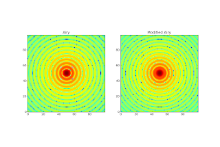
The above image shows the best fit Airy and modified Airy, both in log scale on an identical grid. The modeled PSF was then put through the pipeline to see it recovers the pipeline-derived PSF. The radial profile results are below, but note that this is only one particular realization of the simulation + pipeline.
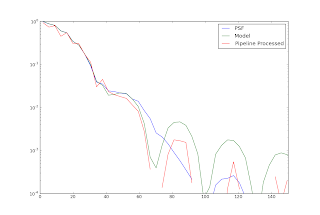
Note that the model matches the first sidelobe in the "observed" PSF pretty well, but both before and after pipeline processing, overpredicts the second sidelobe. There are a few "action items" remaining for this task:
Any thoughts on better models to use? Does this seem like a good idea at all?
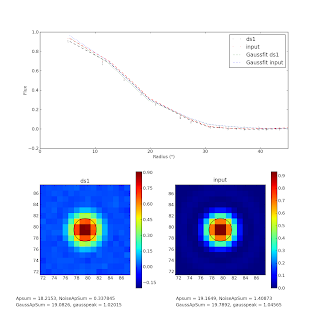
We noted in discussion yesterday that the aperture sum in the (nearly perfectly recovered) is lower than expected even for a gaussian fit of an airy. A Gaussian approximation to an Airy should recover 93.5% of the flux; 6.5% of the power is in the sidelobes of an Airy disk. We recover about 86-88% of the flux in the input point-source map, or about 5-7% short, despite matching the peak to within 2-3%. This discrepancy is partly - but not completely - explained by a slight negative bowl effect: the Gaussian fit has a higher total flux than the aperture sum. Using the gaussian fit value, the recovery is about 90%. A mere 3% missing flux is not too much of a problem - it could still be that the gaussian is uniformly reduced by bowl effects, or perhaps that some flux is not reincorporated into the map (at a very low level) because it is correlated enough to be PCA-cleaned. In the figure, the top panel is the radial profile of the ds1 data (black), the input data (red), and their gaussian fits (see legend). The circles on the labeled images show the FWHM of the fitted gaussian, indicating a good fit. The apertures used for summation are NOT displayed. The sum aperture has a radius of 90" (6.25 pixels) and the "Noise Aperture" has the same area as the sum aperture.
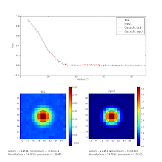
If we redo the analysis with a smaller aperture, the recovery is better: 95% in the central 45". However, now the airy ring cannot account for any lost flux, so it still looks like there's a 5% loss intrinsic in the pipeline.
I'm comparing simulated ds1-ds5 to real ds1-ds5 comparison tests. In the simulated tests, I compare the recovered map after 20 iterations with 13 pca components subtracted to the input map. There are figures showing this comparison for ds1 and ds5 images in addition to one showing the comparison between ds1 and ds5. The agreement is pretty much as good as you could ask for. These simulations are the most realistic run yet. They include a simulated atmosphere that is perfectly correlated between all bolometers excepting gaussian noise, but the relative sensitivity of the bolometers is varied.
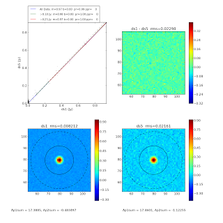


This is what a 'real' ds1-ds5 comparison looks like. The image shown is a "cross-linked" observation of Uranus with downsampling off and on. Note that downsampling clearly and blatantly smears the source flux.

The same image with "beam location correction" looks no better.

The problem is essentially the same with the individual scan directions:


What is causing this difference?
Examining the weights and scales for two individual (real) observations, ds1 followed by ds5, is not particularly telling; there is one additional outlier bolometer flagged out in the ds1 observation, but there is nothing obviously wrong with that bolometer (it may have much lower high-frequency noise than others).


The simulations actually have more discrepant weights, but that doesn't seem to cause any problems:


The timestreams both have similar artifacts:


while the simulated versions really don't:


This is true even when the relative strength of the atmosphere is higher:


I think the most viable candidate is the 'pointing offset' idea, which will take a little work to simulate properly...
Proof that a well-sampled timestream / gaussian is recovered better than a poorly sampled one:


These aren't really the most convincing, since the flux loss is only 1-8% depending on how you count. The atmosphere-included ones have larger flux loss, which is important to understand... WHY does the added noise INCREASE the flux loss? Ugh, unfortunately, there is a perfect counter-example. The first image shows a timestream in which the input map is sampled by 7.2" pixels, which is just shy of nyquist sampling the 1-sigma width of the gaussian (but is fine for the FWHM of the gaussian). The second shows 3.6" sampling of the same. No improvement. The third, very surprisingly, shows significant improvement - but this was an experiment in which the relative scales were allowed to vary.


The first two each had one high-weight bolometer rejected, the last had 12 high-weight bolos rejected. So that's problably the problem....
One of the simplest experiments that can be run is a point-source observed in point-scan mode, i.e. with smaller step-sizes. I've done this for an Airy disk with noise added in the image plan but not atmosphere (some noise is necessary to avoid bizarre artifacts with weighting when you have truly zero signal and zero noise). At a S/N of 500, the noise is pretty minimal, though. It turns out for the 'noiseless' images, the PCA cleaning is the issue... curiously, it varies significantly with iteration. Is it worth trying to debug the PCA cleaning for noiseless timestreams? I mean... they really shouldn't have any correlated information anyway. There is still an outstanding issue where one bolometer gets scaled to be higher than the rest without any apparent reason for doing so. It is also clear that we do not nyquist-sample the pixels with the timestream. However, that doesn't explain a deficiency observed in the ds1 images. Also note that the sidelobes are not picked up at this S/N, but that's not too surprising. And here is the explanation: The peak is missed by about 10% because of finite sampling? Somehow the sampled gaussian nearly uniformly underestimates the gaussian... I think this violates theory a bit.....

Here's the problem shown again:

This is a comparison between the input image and a ds1-sampled image with perfectly correlated atmospheric noise. So there is something in the pipeline that is preventing the peaks from achieving the necessary heights.... I wonder if resampling the deconvolved image onto a higher-resolution grid, then downsampling afterwards, would fix this? Also note that the flux loss increases from 7% to 20% from ds1 to ds5:

It is now possible to make artificial timestreams! First round of tests: For pointing maps with ~21 scans in 15" steps, array angle is approximately negligible. deconv does NOT recover point sources, but reconv does (perfectly) The algorithm starts to decay and produce weird ringey residuals at a S/N ~300. The residuals are only at the 1% level out to S/N ~1000.
Page 1 / 5 »