Preface: This is not a good argument for why astronomy is important now. But it may be in the future. Earth is a limited habitat. Bacteria in a petri dish show the same growth curve as humanity: exponential growth. An exponential curve grows very quickly, but we are in a finite (non-growing) environment. If humanity is to continue its growth, we must find new worlds to inhabit. There is always a moral question of whether we should continue our growth and attempt to conquer significant portions of the galaxy, but we probably won't (and maybe shouldn't) start examining the morality of our survival until it's ensured. Consider what happens if humanity stops growing. Our current economic system is completely dependent on continued growth. The financial markets can't survive unless more wealth is constantly being generated. Interesting calculation to try: Divide the total solar energy input to Earth by the average energy consumed per person, or the minimum energy (theoretically) per person. It's probably not as large as you think when you take into account efficiency factors.
Why can't numpy do duplicate index assignment
AG I want to do drizzling with numpy. It should be trivial, but it's impossible (without a for loop, afaik) instead. In [2]: a = array([1,1,2,2])In [3]: b = arange(5)In [4]: b[a] += 1In [5]: bOut[5]: array([0, 2, 3, 3, 4])In [6]: # but b should really be:In [7]: b[a] += 1In [8]: bOut[8]: array([0, 3, 4, 3, 4])
Why do astronomers have such a strong presence on the web?
I'm not making this a complete post, just a few examples of blogs and websites I'm aware of. But we do have a strong presence on the web - astronomers have an unusually high google ranking etc. Is it just because 'we' were here first ('we' excludes me, I'm just jumping on the bandwagon and getting a free ride)? Examples: Pamela Gay Dr Lisa Science writers who write on astronomy: Dave Mosher
wrapping text around a figure in latex
An example from Devin: %\begin{wrapfigure}{l}{0.5\textwidth} % \vspace{-27pt} % \begin{center} % \includegraphics[width=0.48\textwidth]{nsf_fig3.ps} % \end{center} % \vspace{-27pt} % \caption{\it{}} % \vspace{-12pt} %\end{wrapfigure} 1:16 \usepackage{wrapfig}
Characterizing Precursors to Stellar Clusters with Herschel
C. Battersby, J. Bally, A. Ginsburg, J.-P. Bernard, C. Brunt, G.A. Fuller, P. Martin, S. Molinari, J. Mottram, N. Peretto, L. Testi, M.A. Thompson 2011
The paper includes a careful characterization of the properties of both dense and diffuse regions within the two Hi-Gal Science Demonstration Phase fields (l=30 and l=59). It demonstrated that star formation tracers are more common at higher temperatures, and that IRDCs exist on both the near and far side of the galaxy, where the difference between near and far is around 5-7 kpc.
I helped develop the iterative background subtraction method and contributed to the discussion and conclusions; most of the work was Cara's but my experience with iterative flux estimation from the BGPS pipeline proved useful.
The optically bright post-AGB population of the LMC
E. van Aarle, H. Van Winckel, T. Lloyd Evans, T. Ueta, P. R. Wood, and A. G. Ginsburg
A catalog of post-AGB stars in the LMC, useful in particular because they are at a common distance. Post-AGB stars are quite luminous (> 1000 LO usually), so easily detected in the LMC.
My contribution to this work was years ago; I worked on the SAGE project for a few months at the University of Denver with Toshiya Ueta. I generated a catalog of post-AGB objects and an online catalog with automatic SED plotter. It was a pretty neat project, but I left before I was able to convince others that my catalog was definitive; nonetheless it was eventually used in this publication. As an aside, that was my first foray into data languages, and I ended up using the Perl Data Language long before I learned of python and before I got a free IDL license.
Cross-Correlation Offsets Revisited
Since last time (Taylor Expansion & Cross Correlation,Coalignment Code), I have attempted to re-do the cross-correlation with an added component: error estimates. It turns out, there is a better method than the Taylor-expansion around the cross-correlation peak. Fourier upsampling can be used to efficiently determine precise sub-pixel offsets (matlab version, Manuel Guizar, author, refereed article). However, in the published methods just cited, there is no way to determine the error - those algorithms are designed to measure offsets between identical images corrupted by noise but still strongly dominated by signal. We're more interested in the case where individual pixels may well be noise-dominated, but the overall signal in the map is still large. So, I've developed a python translation of the above codes and then some. Image Registration on github The docstrings are pretty solid, but there is no overall documentation. However, there's a pretty good demo of the simulation AND fitting code here: Tests and Examples The results for the Bolocam data are here (only applied to v2-Herschel offsets):

How does Bolocam data improve greybody fits?


Long wavelength data can be very useful for constraining the value of beta in a greybody fit.
Bolocat V1 vs V2
I've done some very extensive comparison of v1 and v2. The plots below are included in the current BGPS draft, but I'll go into more excessive detail here. ALL plots below show Version 1 fluxes versus Version 2 fluxes using Bolocat V1 apertures. This means there are only two possible effects in play:
- Different fluxes in the v1 and v2 maps
- Pointing (spatial) offsets between the v1 and v2 maps [see http://bolocam.blogspot.com/2012/05/bgps-v2-pointing.html]
Therefore, the plots below are just different ways of visualizing the same information. This holds true despite the fact that different "correction factors" appear in different plots.

Ratios of v2 fluxes to v1 fluxes in the listed apertures. The curves represent best-fit gaussian distributions to the data after excluding outliers using a minimum covariance determinant method
v1 vs v2 with a background subtracted around the source equal to the source area (this was not reported in Bolocat v1, but is a tool Erik implemented so I used it)
v1 vs v2 in 40" apertures, as stated. There are y=x and y=1.5x lines plotted: these are NOT fits to the data! The green line is a Total Least Squares linear fit to the data weighted by the measured errors.
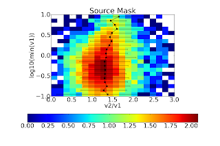
Source Mask "aperture":


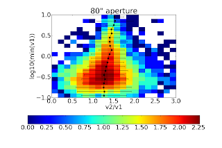
Same as above, but the best fit slope is steeper. The best explanation for the steeper slope (i.e., v2 > 1.5(v1)) is that more extended flux is recovered in v2 around bright sources, therefore in the larger source masks, there is greater flux than would be recovered if a simple 1.5x corrective factor was applied. 80" apertures


Same for 120" apertures:


For all 3 of the 40, 80 and 120" apertures both, the 1.5x correction factor is nearly perfect (agrees to <5%). The background subtraction seems to have different effects depending on aperture size. I welcome Erik to comment on this, but I do not think it is particularly important. The figures below require some explanation. NONE of the circular apertures use background subtraction in this comparison (i.e., compare to the RIGHT column above). These figures are histograms of the flux ratio within a given aperture as a function of flux in the v1 aperture. From bottom to top, the flux in the v1 aperture goes from 0.1 to 10 Jy. The X-axis shows the ratio of the v2 flux to the v1 flux. The black dots with error bars represent the best-fit gaussian distribution to each flux bin. The colorbar shows the log of the number of sources; the most in any bin is about 102.5 ~ 300. In short, there is some sign that the ratio of v2/v1 flux varies with v1 flux. This effect could be seen in the figures above since a linear fit is imperfect. The effect is not very strong. Again, I believe the explanation here is the changed spatial transfer function in v2.


BGPS V2 pointing
BGPS V2.0 pointing offsets relative to V1 and Herschel:

Cumulative Distribution Function of the total offsets.

Histograms of the total offsets.

X-offsets vs Y-offsets (X and Y are GLON and GLAT). The ellipses are centered at the mean of the X/Y offsets and have major and minor axes corresponding to the standard deviations.