
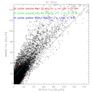

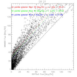
BGPS vs BGPSv2 in Cyg X

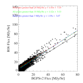
BGPS vs BGPSv2 in IRDC1 (Rathborne)

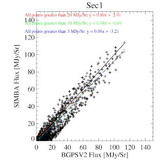


BGPS vs BGPSv2 in l=44 (comparison is SIMBA, not MAMBO)


BGPS vs BGPSv2 in Cyg X


BGPS vs BGPSv2 in IRDC1 (Rathborne)


BGPS vs BGPSv2 in l=44 (comparison is SIMBA, not MAMBO)

The agreement with Motte et al 2007 is now perfect with a vertical ADDITIVE offset instead of the annoying multiplicative offset. An additive offset can trivially be accounted for by a spatial transfer function. As is evident in the difference images, the MAMBO data appears to sit on a plateau.


Cygnus X: BGPSV1:


BGPSV2:


I've finished rederiving the calibration curves self-consistently. These will now be applied to the data....
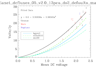
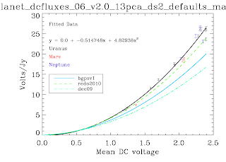


Why did we find a factor ~1.8 in the previous post? Well, for starters we used a calibration curve that was based off of 'masking' and other tricky techniques. The calibration curves below are the first ever produced self-consistently, i.e. using the EXACT same pipeline with the EXACT same parameters as the science data. No hacks were needed to produce these*. The recovered Volts/Jy are substantially higher than BGPSv1 and ALSO higher than the curve used about a year ago in an attempt to explain the v1 flux discrepancy. Remember that a higher calibration curve means a LOWER recovered flux. I haven't finished the check, but odds are pretty good that applying these self-consistent cal curves will reduce the v2 data to be about 1.5.


While no hacks were needed to produce these plots, there were abundant problems. There are far fewer data points than there should be. The problems are manifold, but mostly have to do with the PCA scaling (I think). In some cases, the first scan in an observation was wildly variable. There looked to be an exponential or similar decay (as has been observed in scan turnarounds) at the observation start that took ~3 scans to decay to bring all of the bolometers onto a scaleable curve. This is a HUGE problem, because the assumption that the dominant signal is atmosphere is badly violated in this situation - the signal becomes electronics-dominated. The first PCA component is then an ugly step-function. With these first scans flagged out, the whole problem goes away, but that's a painful manual process. Automating it MAY be possible, but also risky. In other cases, particularly September 4th 2007, the atmosphere appeared to be negligible! While the atmospheric optical depth probably was not, if it was extraordinarily stable over the course of ~10 minutes, again we experience severe problems. A stable atmosphere means no atmospheric variation, which means that ACBOLOS is just noise (plus Uranus signal). Ironically, this is very bad for calibration - it means there is no common signal on which we can calibrate the bolos' relative sensitivities. This problem doesn't seem to affect science data, probably because there's no such thing as 45-minute stable atmosphere (especially when you're following rising/setting sources). If I REALLY need that data, I could snag the relative scalings from a science field and apply them to the cal data... honestly that's not a bad idea in general... hmm... Well, we'll explore that later if I have time, that will take days to implement.
ds1 and ds5 agree pretty well with the recent upgrades to delining and deconvolution. However, there are still counterexamples, e.g. 101208_o13, in which ds5 < ds1:


The 'fitted' values agree better than the 'measured' values now that NANs are treated properly. Spent a few hours today trying to figure out if weighting can explain the difference between ds1 and ds5; it appears to make up for most of it so I'm doing some more experiments. Why is there so much parameter space? Why can't weighting just work? It doesn't.... also wasted a few hours trying to write a python drizzling algorithm, which unfortunately is impossible so I had to resort to an inefficient for loop. Finally got some minor results. It really looks like there is a trend pushing up the recovered flux (i.e. higher volts/Jy) for ds5 over ds1. There is a discrepancy between map types for ds1 but not for ds5, which is actually backwards from what I would have expected, since ds1 will get better-sampled maps.


Luckily, the difference between peak fitting and "measuring" results in very small (insignificant) changes to the calibration curve (recall fitting is direct gaussian fitting; 'measuring' is using the gaussian-fit width and total flux in an ellipse to infer a peak assuming a point source):


Since this work has all been done for the 'bootstrapping' observations that are supposed to tell us if different map sizes are compatible, I have included the map sizes in the diagrams now. However, to really understand the ds1/ds5 difference, there are much better data sets, which I'm now reprocessing using the new and improved methods. (the Whole BGPS is also processing with the new methods in the background, though since the methods are being updated live there may be more changes and it will have to be re-run.... initial looks at W5 are BAD but L030 is GOOD (bordering on amazing))
I looked very closely at the timestream and maps of 101208_o11 and had a pretty hard time figuring out why the data were different, but it looked like the data really did differ on a point-by-point basis (according to pyflagger). The only conclusion I was able to draw is that the scaling must be off. I realized that the scaling was being done before delining. I moved scaling from readall_pc to premap, and it brought at least this one source into agreement. Time to run ds1-ds5 comparisons again! (this means that ds1 data MUST have deline run on it, but ds5 data doesn't really need it) Here are examples of ds1 and ds5 timestreams, with and without scaling, and ds1 with and without delining:


I've concluded, based on previous posts http://bolocam.blogspot.com/2011/02/downsampling-why-is-dec-2010-different.html, http://bolocam.blogspot.com/2011/03/revisiting-calibration-yet-again.html, and http://bolocam.blogspot.com/2011/03/workaround-for-individual-maps.html, that ds5 is a problem primarily for undersampled images, i.e. those taken in the normal mapping mode. This makes bootstrapping a bit tricky.
There are two options:
- Map Uranus and AFGL 4029 both in Volts and figure out what flux density AFGL 4029 must have to lie on that curve
- Map Uranus and compute a calibration curve, apply that calibration curve to AFGL 4029, and then compare derived flux densities.
Both have the major problem that the individual AFGL 4029 maps will forcibly be undersampled if I use ds5 data (which is normally OK, according to the first paragraph). In the second case, it is possible to co-add the images and get around the under-sampling issue, while in the first case it is not because of the dependence on total loading (MEANDC).
The real problem is that the whole goal of these observations was to compare the different observing methods and see if they agree (1x1, 3x1, pointing, etc.) since the pointing-style observations were used to calibrate the others. But if the 1x1s are just straight-up unreliable, how can we do the comparison? I think the co-added AFGL 4029 is the only option, but then how do I test if it's correct? It would be really nice to have AFGL 4029 observed with both scan types...
Alright, onto the data. After last week's fix of the bad bolos, I really hope ds1 and ds5 agree. However, first glance at the cal curves says they don't. ds1 and ds2 agree, but ds5 is different.
After checking them out with ds9 *ds[15]*13pca*_map10.fits -scale limits -1 1000 -log -cmap hsv -match colorbars -match scales -match frames wcs &, it appears that the _mask_ data is all... wrong, somehow. That's OK, I want to discard the mask data anyway, so I'm happy to NOT spend time debugging it.
Even after careful examination showing that the fits look good - and noting that the fluxes look pretty much the same - the calibration curves still look rather different. Unfortunately I had to spend 3 hours debugging IDL plotting commands; I want to show the fits each time and save them as postscripts. What does "xyouts" with "/device,/normal" do? I thought that should plot x,y text at the coordinates specified in the plot window... but no, that is JUST /normalize.
Anyway, realized that centroid_map treated NANs as zero. Added ERR keyword (with a reasonable estimate of the error) in centroid_map to ignore NANs. It looks like improper treatment of NANs is responsible for a lot of the scatter seen in the calibration plots.
There is a substantial difference between the "fitted" peak and the "measured" peak (the latter computed by taking the sum of the pixels divided by the area of the fitted gaussian). It looks like the "measured" version is more robust, at first glance. However, unfortunately, for 101208_o11, the difference between ds1 and ds5 exists in both quantities. I will have to examine timestreams now... ARGH.
Well, the timestreams show... that indeed the model is lower in ds1, but not why. The "remainder" (new_astro; the stuff that never gets incorporated into the model but DOES get incorporated into the map) appears to be the same in both. Similarly, there is little to no flux in the PCA atmosphere, so it's not simply being cleaned out. Where is the flux going or coming from?


The recent hiatus for paper revisions has, unfortunately, come to an end. Re-examining my work, I did quite a lot but encountered many dead-ends. First, we would very much like to use an *identical* reduction process on both the calibration data and the science data. That way, we could feel very confident that the reduction process isn't introducing any weird artifacts. Unfortunately, I discovered early on that using ds5 data, 13 pca components, and n>1 iterations resulted in strange shape and flux conservation failures. These errors do NOT occur in co-added maps; they are unique to single-observation scans (though I don't recollect whether 2 scans is enough or if you need more). I spent many hours banging my head against this problem and have never gotten a satisfactory solution. But perhaps it's time to approach it again. The map00 images look MUCH rounder and generally better than the map10 images. So, the problem I need to examine is the iterative process. Why does it fail for single images? Is it something about the noise properties? model00 looks fine... what gets put into the timestream? Examining timestreams is a terrible and horrendous process... but what else can I do? The next step will be to examine the timestreams of a particular observation. I think a good choice is 101208_ob7; the next observation, 101208_ob8 was a large-area map and it looks fine (i.e., it improves with iteration). So I can start looking at the effects of polysub, iteration, etc. on this particular source. Of course, the stupid trick with the pipeline - every time - is that "fixing" a problem for one source has a nasty tendency to break it for all other sources. That's why there are so many flags that can be passed around. Still, this is the approach I have to take...
Background: Downsampling is performed using Old Pipeline code called process_ncdf. All BGPS data was downsampled by a factor of 5 before mapping because of data size concerns. I did this 'blindly' (i.e., just accepted that I should) because James said I could. However, I had previously noted that the pointing files could not be done with downsampled data because the beams 'looked funny' or something along those lines; it may also have been a simple map sampling issue in which not all pixels were filled with a downsampled image. Anyway, I decided to go back and quantify the effects. The plots below are from the single "pointing-style" observation of OMC1 from 2009. The units are volts. 'ds1' indicates sampling at 0.02 seconds, 'ds5' indicates sampling every 0.1 seconds. The scan rate was 120"/s.

The beam sizes were measured from the autocorrelation maps. However, because there is structure on many scales in this map, I had to use a rather ad-hoc method to remove the correlated structure. I fitted a gaussian to the elliptical northwest-southeast structure, removed it, then fitted a gaussian to the remaining circular thing in the center, which is approximately the beam. If I fit the "beam" gaussian with an ellipse, I get: Beamsize 1_1: 36.15,26.23 Beamsize 1_5: 48.39,30.21 With a circle: Beamsize 1_1: 29.51 Beamsize 1_5: 35.31

The ds1 and ds5 images compared.

The PSDs of the two images (on identical grids). Note that ds5 loses power at small spatial scales, 50% at 40"!
The pixel-pixel plot with a fit that shows a 10% overall flux loss (best-fit).
I've started looking at PPS fields to see if I can glean any additional information about the "flux discrepancy" from them. However, the results are, as usual, unenlightening. There is no consistent increase in flux when 3 PCA components are used instead of 13 PCA components - very plausibly an indication that 13 PCA is not too much to subtract because it's only atmosphere. Similarly, there is no obvious benefit to using a quadratic sky estimator instead of a PCA estimator. I'm using aperture photometry (without background subtraction) on identical fields to perform these comparisons. I've selected (arbitrarily) the l357pps source as my comparison source. The next step (ongoing) is to compare to the co-added maps and crosshatched large-scale maps of the same field. (next step) PPS < single cross-hatched large-scale observation pair < 13PCA full combined map < 3PCA full combined map. Unfortunately, this result implies that the small maps under-recover flux, which suggests that the large maps are too bright, which is the opposite of what we expect. Additionally, lower noise -> more flux recovered? When background subtraction is included, the 3PCA and 13PCA fluxes match nearly perfectly. Despite the failure of this test (PPS < full field), I will do a systematic comparison of PPS sources with 0PCA + masking to the large fields in the hopes that doing so can provide a legitimate estimate of the "scale factor" from treating small and large fields differently.
Page 1 / 2 »