To convert from MIRIAD map files to FITS, use:
miriad% fits in=h2comos1.clr out=h2comos1.fits op=xyout
To convert from MIRIAD map files to FITS, use:
miriad% fits in=h2comos1.clr out=h2comos1.fits op=xyout
From Andrew Walsh, a script to install MIRIAD:
wget ftp://ftp.atnf.csiro.au/pub/software/miriad/miriad-common.tar.bz2
wget ftp://ftp.atnf.csiro.au/pub/software/miriad/miriad-linux64.tar.bz2
bzcat miriad-common.tar.bz2 | tar xvf -
bzcat miriad-linux64.tar.bz2 | tar xvf -
cd miriad
export MIR=$PWD
# define the MIR variable in your bashrc
echo "export MIR=$MIR" >> ~/.bashrc
sed -e "s,@MIRROOT@,$MIR," scripts/MIRRC.in > MIRRC
sed -e "s,@MIRROOT@,$MIR," scripts/MIRRC.sh.in > MIRRC.sh
chmod 644 MIRRC*
# Put these into .bashrc, or call them each time you want to run MIRIAD
. $MIR/MIRRC.sh
export PATH=$PATH:$MIRBIN
My boss asked a great question at our first weekly ESO-python tutorial session: What does a good ipython debugging workflow look like?
The one advantage I had found in IDL was that everything is a script, which means that everything can be debugged in the same way: add a stop statement at the relevant line of code. Of course, that debugging model breaks apart badly once you start writing complex programs and using things like common blocks.
In ipython, there is a beautiful debugger that is far more feature-rich than the IDL equivalent. It can be activated simply:
%pdb
will toggle the interactive ipython debugger. Then, if you run into a code crash, you will be dumped out at an ipdb> prompt, with access to a fully-functional python prompt in the local namespace / environment of the crash point. You can also move up and down the function hierarchy with the u and d commands.
The existence of the ipdb debugger suggests a natural approach for those familiar with IDL debugging: simply add a raise statement wherever you would normally have put a stop statement. There are a few key differences, however: in IDL, you could just .continue to run the rest of the code as if no stop occurred; in python the same is not possible with the default ipdb.
However, the ipdb package allows the insertion of breakpoints just like in IDL:
import ipdb; ipdb.set_trace()
From within one of these breakpoints, the .continue command will continue on to the next breakpoint, as you might expect. The n and s commands will go to the next line in the code, while s will allow you to drop into called functions (how?)
Postmortem debugging is also awesome. If you have run a command and gotten a traceback, you can retroactively enter the debugger:
%debug
but as with the normal traceback debugger, one cannot continue afterward.
Python code is typically distributed in packages managed with a setup.py script. These are the most convenient way to install, use, and distribute code, but they are not ideal for debugging.
When debugging a normal script, something you could run by invoking
python myfile.py
or
%run myfile.py
# in the local namespace
%run -i myfile.py
# with the python debugger active:
%run -d myfile.py
can easily be debugged by running it line-by-line. The documentation can be accessed via the %magic command.
For debugging "compiled" packages, though, more thought is needed.
If you are working on your own package, you can use setuptools to enable the python setup.py develop command, which installs a symbolic link to the source code directory - meaning any changes you make are immediately reflected in the python source path. This does not mean that any changes are recognized in the local python environment, though!
If you are in an active ipython session, you need to reload packages to see their results. As far as I know, you can never "reload" the source code underlying an already-instantiated class, so you have to remake any class instances you want to examine.
The reload command is tricky to use. You will only see changes to the source code if you import the exact package in which the code is stored. For example, if you have a file structure like this:
mypackage/
__init__.py
core.py
and you do reload(mypackage), that will effectively reload only the source code in __init__.py. If the code you want to use is called myfunction and it lives in core.py, you can reload that source code by doing reload(mypackage.core). Reloading mypackage may have no effect. So the key for developing packages is finding the right module to reload!
IPython has a deepreload package intended to recursively reload functions; it may work but I had trouble in the past.
It's generally much better to have a test suite enabled with unit tests for each component of your code. This is the approach adopted by most open-source projects and many industrial code developers.
Tests are invoked with the command py.test with a variety of command options. Among my favorites are py.test --tb=short, which gives a much less verbose traceback, py.test --pastebin=failed, which posts any failure results to pastebin for easy sharing, py.test -p packagename (or python setup.py test -P packagename in astropy) to select tests for a specific package. A great deal more options can be found in the pytest docs.
A test suite, if properly constructed, can also be run from with in ipython:
import astroquery
astroquery.test('eso')
Some useful related links:
Installing astrometry.net is all about navigating dependency hell.
Requirements:
- libpng
- libtiff
- libjpeg
- netpbm (requires above 3)
To install netpbm, a recent version - NOT the stable version - is required, which means navigating throught 3-4 layers of links including a sourceforge build-my-tarball link.
To compile astrometry.net-0.50:
ARCH_FLAGS="" make -j 8
To compile cairo, I had to install pixman (no problem) the setup a PKG_CONFIG_PATH:
PKG_CONFIG_PATH=/usr/local/lib/pkgconfig ./configure
Can we characterize "hub" clumps vs "filament" clumps by examining their azimuthal column density profile? Filaments would have two-peaked structures, hubs many-peaked, and spherically symmetric "isolated" clumps would be peakless.
As you might expect from numerous blog posts and the general difficulty people have always experienced upgrading mac OS versions, Mavericks caused some truly hideous issues.
The only really "new" issues specifically for Mavericks relate to app nap. The main solution is minrk's appnope. Otherwise, command line options like defaults write <app domain name> NSAppSleepDisabled -bool YES are required if the button is missing from Mac's Get Info pane.
I tried installing the conda stack to get python running quickly. This worked to an extremely limited degree: the TkAgg shipped with anaconda links to XQuartz, which is highly undesirable for a number of reasons. This meant that matplotlib plots showed up as X11 plots. With the Mac OS X backend, the windows failed to show up in the Dock and therefore were totally unusable (though they did look OK).
I am still using conda to maintain multiple parallel versions of python for testing. However, I went back to my typical install-from-source approach.
To get the matplotlib backends to interact nicely with apple, you need to install them using the /Library version of python
# this had to happen sometime early:
$ xcode-select --install
$ wget https://pypi.python.org/pypi/pip#downloads
$ tar -xzvf ~/Downloads/pip-1.5.2.tar.gz
$ cd pip-1.5.2
$ /Library/Frameworks/Python.framework/Versions/2.7/bin/python setup.py install
$ /Library/Frameworks/Python.framework/Versions/2.7/bin/pip install virtualenv
$ cd
$ /Library/Frameworks/Python.framework/Versions/2.7/bin/virtualenv virtual-python
After this, I was surprisingly able to install everything in the python stack with no hitches. Obviously, that could not possibly last.
While matplotlib and numpy worked fine, scipy had problems.
ImportError: dlopen(/Users/adam/virtual-python/lib/python2.7/site-packages/scipy/integrate/_odepack.so, 2): Symbol not found: __gfortran_internal_free Referenced from: /Users/adam/virtual-python/lib/python2.7/site-packages/scipy/integrate/_odepack.so Expected in: flat namespace in /Users/adam/virtual-python/lib/python2.7/site-packages/scipy/integrate/_odepack.so
This terrible error led me back to re-compiling scipy. I tried installing with hpc gfortran, but that didn't work at all, first apparently because of linking errors in numpy. When I investigated numpy, I found that the compilers apparently don't work at all:
C compiler: /usr/local/bin/gcc -DNDEBUG -g -fwrapv -O3 -Wall -Wstrict-prototypes -arch i386 -arch x86_64 ... RuntimeError: Broken toolchain: cannot link a simple C program
I had to give up on that, and then googling returned no results at all, which I thought was a bit weird. Scipy seems to want gcc and g++ 4.2, even though they're years old. I had to find those and gfortran-4.2 somehow, but the old site that used to serve them seems to have lost the files! They had an older version, though, which appears to work. Scipy is a scary install.
XQuartz is not well-behaved on Mac OS X 10.9. First, on retina machines, it does not display well. Second, and much more important, it does not work on external monitors. Apparently this can be worked around by turning off "Displays have different spaces" in Mission Control, but so far that has had no effect for me.
In the process of creating W51 data cubes from the GBT mapping data (project GBT 10B/019), I've had to deal with a lot of bad data.
Some of the bad data comes from misbehaving electronics. All I can say is that they were misbehaving, not how or why - the data from one polarizaiton simply disagrees with the other polarization and feeds spontaneously and for no apparent reason.
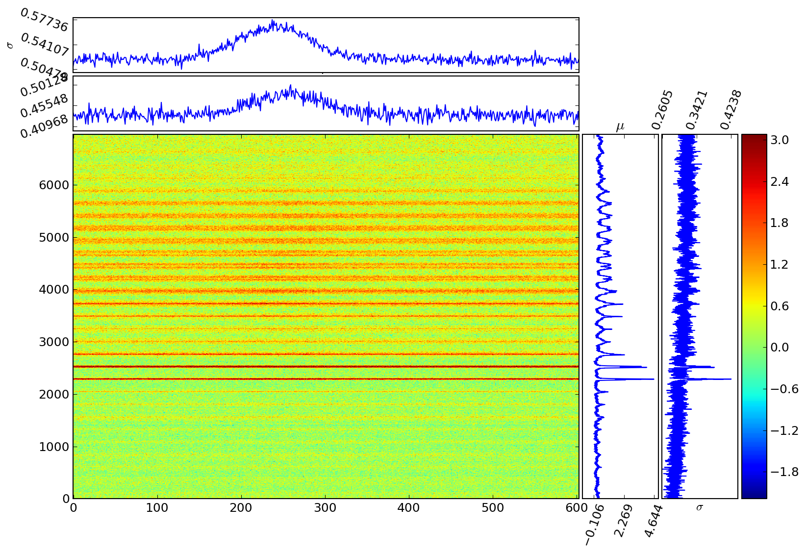
I've implemented a waterfall diagnostic plot to help examine the data, it is in my mpl_plot_templates repository: imdiagnostics.py.
A good waterfall looks something like this:
The line plots show the average and standard deviation along each axis; the right side effectively shows timestream continuum data while the top plots show a time-averaged spectrum. This plot is good in that there are clearly signals detected as the scan crosses continuum sources and there is a strong Helium Alpha line detected in the average (though there's no way to read that it's Helium fromt he data as presented). Notably, the noise correlates with the continuum brightness - this is expected; higher TSYS leads to higher noise.
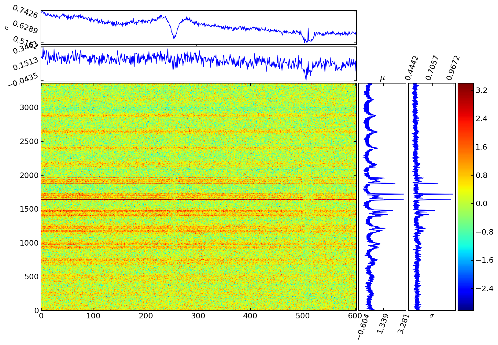
This is an example of a data set with some extremely irritating artifacts. There are apparent absorption lines throughout the spectrum: they are not real. This is a particularly irritating problem because I had resolved it once in the not-too-distant past, but I can't figure out how!! Most likely, I just removed the data from the maps, but that SHOULD be in the code history (git) and is not.
In order to regrid an image, you need some target reprojection. The simplest way to acquire such a reprojection is by extracting it from another image, e.g. a FITS image
(I use >>> to indicate the CASA <#>: prompt here because it allows you to copy & paste the code into CASA)
>>> header = imregrid(imagename='file.image', template='get')
This header will be a python dictionary with two keys, csys, which specifies the coordinate system, and shap, which gives the shape.
If you want to write up your own FITS header and you don't have a FITS file with those exact coordinates, you can use the header_to_template convenience tool in casa_tools.
>>> from casa_tools import header_to_template
>>> from astropy.io import fits
>>> fits_header = fits.Header.fromtextfile('my_header.hdr')
>>> header = header_to_template(fits_header)
In order to regrid the file, you then need to pass in the image name and template to imregrid.
>>> imregrid(imagename='file.image',
... template=header,
... output='file_regrid.image')
If your input image's header did not include a 'telescope' keyword, CASA will complain:
2013-12-18 16:46:33 SEVERE imregrid::ImageRegrid::regrid (file /opt/casa/release-4_1_0-release-1/darwin64/include/casacore/images/Images/ImageRegrid.tcc, line 118) Cannot find the observatory name UNKNOWN in the CASA
You can add the keyword to the header yourself:
>>> imhead('file.image',
... mode='put',
... hdkey='telescope',
... hdvalue='Arecibo')
- Sebastian Muller's presentation (page 16)
- imregrid docs
If you want to perform analysis on a FITS file in CASA, you first need to import it into .image format.
importfits('file.fits','file.image')
If this works, great! You can move on. CASA will treat NaN values in an image as 'masked'.
There may be issues with FITS headers. CASA respects a large number of header keys (reference).
There are many ways to edit a FITS header. One of the most straightforward to use is edhead. Otherwise, one can use CASA's imhead
CASA Keyword | FITS keyword | Description |
beammaj | BMAJ | Major axis of the clean beam |
beammin | BMIN | Minor axis of the clean beam |
beampa | BPA | Position angle of the clean beam |
bunit | BUNIT | Brightness unit (K, Jy/beam, etc) |
cdeltn | CDELTn | Pixel size, nth axis (max n is 4) |
crpixn | CRPIXn | Pixel coordinate of reference point, nth axis |
crvaln | CRVALn | Pixel location of reference point, nth axis |
ctypen | CTYPEn | Axis name, nth axis. For FITS, this includes the projection |
cunitn | CUNITn | Pixel units, nth axis |
datamax | DATAMAX | Maximum pixel value in image |
datamin | DATAMIN | Minimum pixel value in image |
date-obs | DATE-OBS | Date of the observation |
equinox | EQUINOX | Reference frame for directional coordinates |
imtype | Image type: intensity, | |
minpos | Position of the minimum value (world unit) | |
minpixpos | Same in pixel (array) | |
maxpos | Position of the maximum value (world unit) | |
maxpixpos | Same in pixel (array) | |
object | OBJECT | Source name |
observer | OBSERVER | Observer name |
projection | CTYPEn | Image projection ('SIN','TAN', or 'ZEA') |
reffreqtype | Reference frame for the spectral coordinates | |
restfreq | RESTFREQ | Rest Frequency |
shape | NAXISn | Number of pixels along each axis |
telescope | TELESCOP | Telescope name |
What does it mean if you get this sort of error?
CASA <1>: importfits('file.fits','file.image') 2013-12-18 13:06:18 WARN importfits::FITSCoordinateUtil::fromFITSHeader The wcs function failures are too severe to continue ... 2013-12-18 13:06:18 WARN importfits::ImageFITSConverterImpl::FITSToImage (file /var/rpmbuild/BUILD/casapy-stable/casapy-stable-42.0.26945/casacore/images/Images/ImageFITSConverter.tcc, line 71) No proper coordinate system defined in FITS file. Using dummy linear system instead.
First, go to the casapy-yyyymmdd-hhmmss.log file and look at the errors.
2013-12-18 13:06:18 INFO importfits::FITSCoordinateUtil::fromFITSHeader celfix incurred the error Inconsistent or unrecognized coordinate axis types 2013-12-18 13:06:18 INFO importfits::FITSCoordinateUtil::fromFITSHeader spcfix incurred the error Inconsistent or unrecognized coordinate axis types 2013-12-18 13:06:18 INFO importfits::FITSCoordinateUtil::fromFITSHeader cylfix incurred the error Inconsistent or unrecognized coordinate axis types
In my case, the error turned out to be that CTYPE3 was set to RADI-LSR, while it should be VELO-LSR to be recognized by the CASA system. The velocity convention is, unfortunately, lost.
Sgr B2 is the most massive gas clump in our Galaxy. It's about 100 pc away from Sgr A*, the black hole at the center of the Galaxy. It is forming stars prodigiously, and has extreme properties in many regards.
In many physical aspects - mass, luminosity, velocity dispersion, temperature - the Sgr B2 region is similar to "proto-cluster clumps" seen in other galaxies, e.g. the Antennae galaxies.
There are plenty of mysteries about Sgr B2, including its extraordinarily diverse chemistry and its peculiar kinematics.
I'm raising a sort of new one. There appears to be a hole next to Sgr B2, towards the southeast in Galactic coordinates. It appears as a relatively empty spot in the dust continuum bands. It doesn't seem to be filled in with anything in particular.
Note the slider here: you can view Sgr B2 at any wavelength where I have data. The green circle highlights the major deficiency that is evident in all dust-containing bands. There are other "minor" deficiencies elsewhere.
It is tricky to interpret this: I don't think the absolute flux densities in any of the millimeter observations are perfectly trustworthy because of their proximity to the extremely bright Sgr B2 point sources.
Additionally, this gap is not perfectly evident in NH3 or CO. In the HOPS NH3 maps, there is a relative lack of emission at ~56 km/s - relative to neighboring regions; this is actually the peak of the line profile extracted from the ellipse!
This is in contrast to the central "Gas Hole" which has been noted by others; it exists in CO and NH3. There is almost certainly some NH3 self-absorption involved. The "Gas Hole" coincides with the peak in other gas species and the peak in the dust emission, so it really seems to be a different phenomenon, having to do with line-of-sight confusion and excitation conditions.
The one feature of the "dust gap" that distinguishes this part of Sgr B2 from the other regions surrounding it is that 8 micron emission can readily be observed here. A little 24 micron emission is in the gap as well, but not as much as the 8 micron. The 70 micron emission is quite weak, but not really deficient. Perhaps in this region, very small grains are more common than in its surroundings?
There's a lot more hypothesizing to be done here.