Made with this code and graphviz.


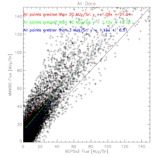

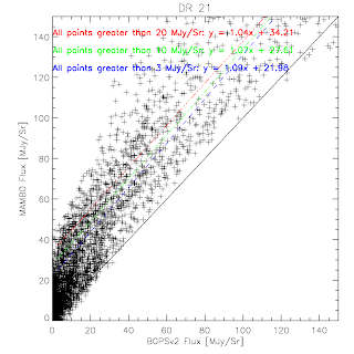
BGPS vs BGPSv2 in Cyg X

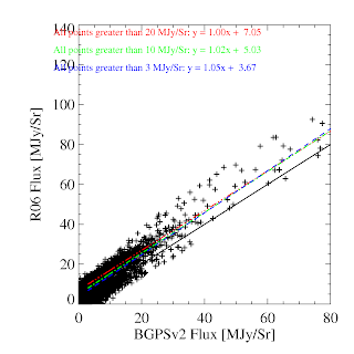
BGPS vs BGPSv2 in IRDC1 (Rathborne)

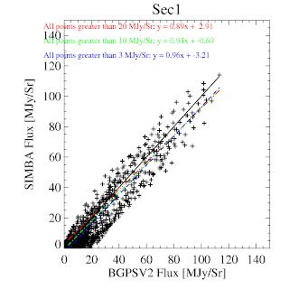


BGPS vs BGPSv2 in l=44 (comparison is SIMBA, not MAMBO)

Check to make sure original fits were/were not forced through 0,0
The agreement with Motte et al 2007 is now perfect with a vertical ADDITIVE offset instead of the annoying multiplicative offset. An additive offset can trivially be accounted for by a spatial transfer function. As is evident in the difference images, the MAMBO data appears to sit on a plateau.


Cygnus X: BGPSV1:


BGPSV2:


I re-examined the Bolocat data on l351 after re-running the pipeline with the new calibration curve. The change wasn't all that great. See this post for a brief description of the procedure. In the data below, I've fit the residuals as a function of v1.0.2 flux density in an aperture (source mask) with a line. The slope of the line should ideally be zero - that would indicate a multiplicative offset is an acceptable correction. Nicely, in the 40" aperture case, I see no reason to exclude the m=0 case. For the most reliable data - the 13pca - the slope is rather small and the "correction factor" is disturbingly close to what we recommended (1.5). We have no right to be that lucky...

...and so perhaps wer are not. The source mask includes more area and therefore is more sensitive to extended flux recovery. The slopes are not consistent with 0 - just look at the data above and below 2 Jy to see that there is a difference. The multiplicative correction of 1.5 is decent for a pretty wide range of flux densities, but is inadequate for the brightest sources. This is somewhat interesting... it implies that the brightest sources also lie on the highest backgrounds.

You might note that the brightest source has a smaller correction factor in both apertures. It's not clear why that is the case, but I don't think it's enough to call it a trend yet - wait for the full 8000-source comparison first. Why is there so much scatter? Not entirely clear, but the scatter is primarily at low S/N.
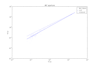

Here are the same for all of the data reduced up to this point:


I've finished rederiving the calibration curves self-consistently. These will now be applied to the data....
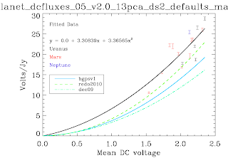
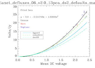


Why did we find a factor ~1.8 in the previous post? Well, for starters we used a calibration curve that was based off of 'masking' and other tricky techniques. The calibration curves below are the first ever produced self-consistently, i.e. using the EXACT same pipeline with the EXACT same parameters as the science data. No hacks were needed to produce these*. The recovered Volts/Jy are substantially higher than BGPSv1 and ALSO higher than the curve used about a year ago in an attempt to explain the v1 flux discrepancy. Remember that a higher calibration curve means a LOWER recovered flux. I haven't finished the check, but odds are pretty good that applying these self-consistent cal curves will reduce the v2 data to be about 1.5.


While no hacks were needed to produce these plots, there were abundant problems. There are far fewer data points than there should be. The problems are manifold, but mostly have to do with the PCA scaling (I think). In some cases, the first scan in an observation was wildly variable. There looked to be an exponential or similar decay (as has been observed in scan turnarounds) at the observation start that took ~3 scans to decay to bring all of the bolometers onto a scaleable curve. This is a HUGE problem, because the assumption that the dominant signal is atmosphere is badly violated in this situation - the signal becomes electronics-dominated. The first PCA component is then an ugly step-function. With these first scans flagged out, the whole problem goes away, but that's a painful manual process. Automating it MAY be possible, but also risky. In other cases, particularly September 4th 2007, the atmosphere appeared to be negligible! While the atmospheric optical depth probably was not, if it was extraordinarily stable over the course of ~10 minutes, again we experience severe problems. A stable atmosphere means no atmospheric variation, which means that ACBOLOS is just noise (plus Uranus signal). Ironically, this is very bad for calibration - it means there is no common signal on which we can calibrate the bolos' relative sensitivities. This problem doesn't seem to affect science data, probably because there's no such thing as 45-minute stable atmosphere (especially when you're following rising/setting sources). If I REALLY need that data, I could snag the relative scalings from a science field and apply them to the cal data... honestly that's not a bad idea in general... hmm... Well, we'll explore that later if I have time, that will take days to implement.
For this experiment, I ran Bolocat on all of the v1 and v2 images using the source masks Erik derived for v1. I then compared the derived fluxes using both aperture photometry (as defined in bolocat) and the mask sums.
First, note that the object_photometry code Erik wrote does NOT do background subtraction - this is important for understanding non-multiplicative offsets between v1 and v2.
I fit a 2-parameter model (a line) to the v2 vs v1 plots using two methods. The simple linear-least-squares method is one we're all familiar with, and it gives semi-reasonable results, but is NOT statistically robust when there are errors on both axes. The other fit method used was Total Least Squares, which is approximately equivalent to Principle Component Analysis with 2 vectors. It uses components of the singular-value-decomposition to determine the best fit. The fits returned by TLS should be more robust, though the additive offsets need not be.
Conclusion: Our factor of 1.5 looks like it was pretty accurate. For 40" apertures, the best fit is ~1.56, which is easily within the error bars. Luckily, for 40" apertures, there is no apparent need for an additive offset (I'm pretty sure the uncertainty on the measured offset is larger than the offset, though statistically that is not the case), which would complicate things.
However, for the source mask, there is a greater scaling factor and a very substantial offset. This implies that the peaks in v2 are brighter by a large factor, but the backgrounds in v2 are actually lower than in v1 (though please do check my reasoning here). I'm really not sure what to make of the difference between source mask and aperture yet, though... there's probably something significant in the source mask being forced to pick positive pixels. (and peppered pickles)


Some positive results. v2 is uniformly higher than v1, but at nearly 1.8, not 1.5. Some of this could be because of a different calibration curve (which is worth checking on; I'll do that later).
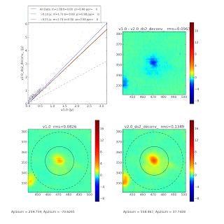


While the pixel-to-pixel comparison yields values ~1.75, the aperture photometry is perhaps even more severe:


Those are a difference of a factor of 2.5, which is rather enormous.
So the code to add point sources to the maps and perform basic aperture photometry has started working to the point where I can share some results.
For maps with no underlying sky structure, only point sources, recovery is very nearly perfect, with PearsonR coefficients essentially equal to 1 until the peak amplitude of the point sources drops below 2.0 (and even then they only drop to ~0.997)
Below is a sample of the difference residual of output-input flux vs input flux for 40", 80" and 120" apertures

flux vs input flux will show just how correlated these are:

Note that for the blank maps, these are taken from simulations using a power law distribution of point sources from 0.1 to 2.0 Jy in magnitude (if we allow the range to extend above 2.0 Jy, the recoveries become even more closely correlated.
As for simulations with background sky structure we see similar patterns for the most part, however a few interesting pieces appear:
For the 4 different source ranges I ran, the 80" aperture had the highest pearson r coefficient across all simulations. Generally sitting around 0.95 with the 40" and 120" apertures floating from 0.75-0.9. This may be a fluke, however, I need to run more simulations to see if this is reproducible with other seeds.
Also, in the difference residuals we can clearly see an underrecovery of flux as input flux increases, which we should probably work to quantify, as seen by this example:
