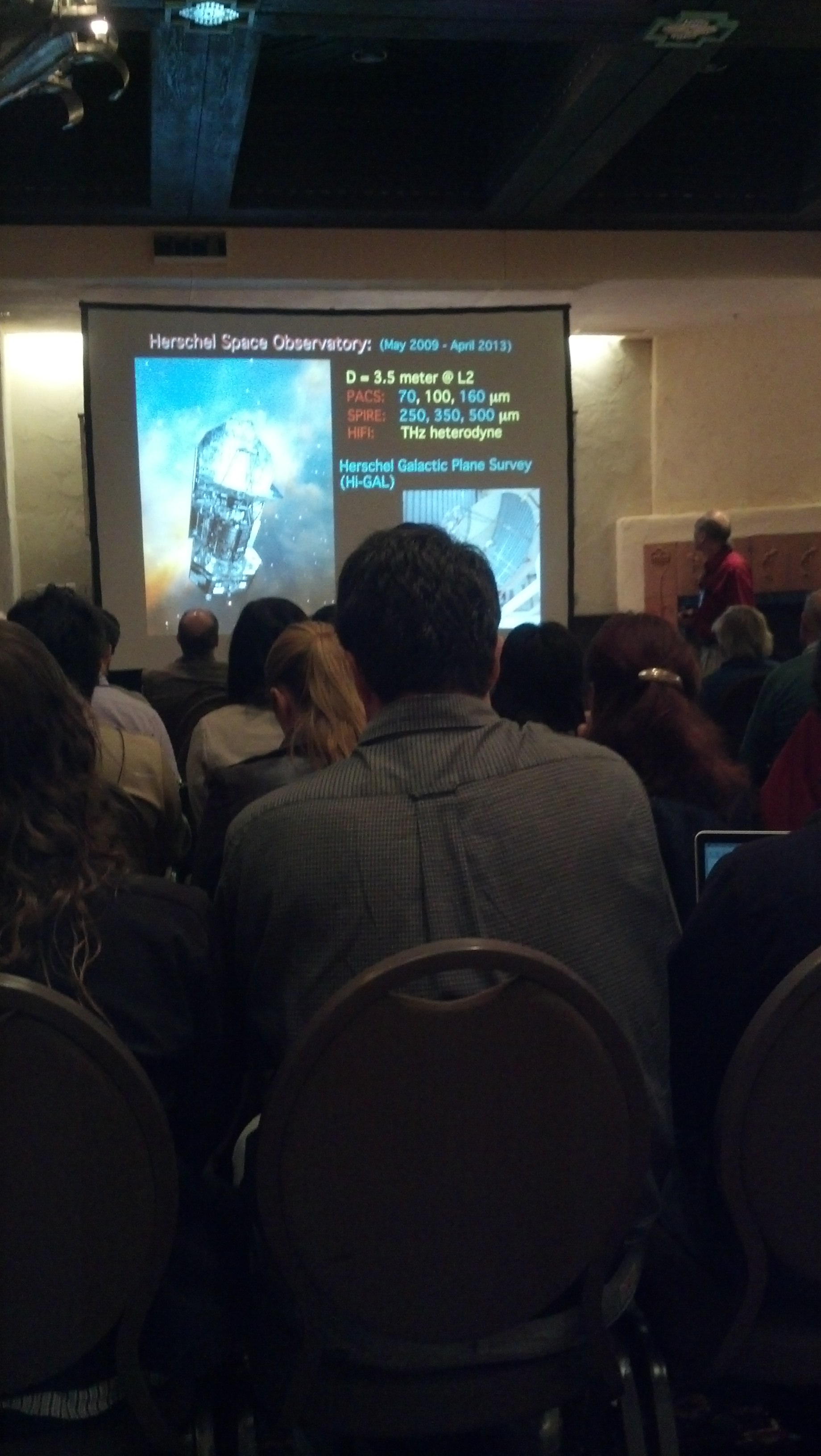
- TeV observations
- scintillation in air (Cherenkov)
- Hadron detection
- watching for light showers
- HESS camera is huge: 1.5m across (fast photometers)
- HESS, VERITAS, MAGIC dominate
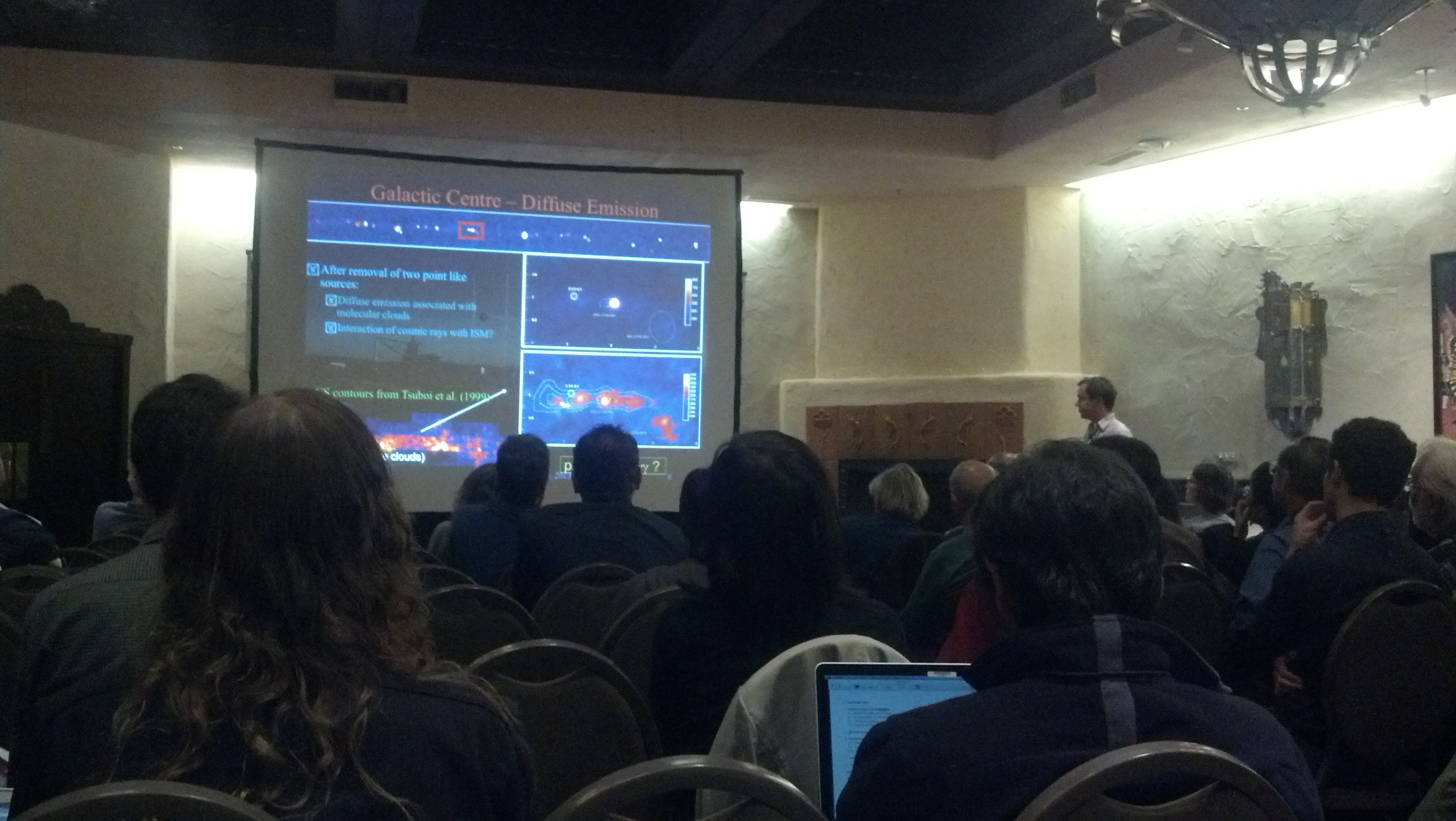
- Galactic Center
- high energy density (100 eV cm^-3)
- dense GMCs & starburst activity
- HESS CMZ good...
- VERITAS CMZ 18-sigma in 46h
- HESS, mol clds trace similar areas
- Local excess of 10 TeV -> requires local source of CRs
- Correlation between mol clds great in Sgr B, Sgr A, but poor in Sgr D + no TeV emission at |l|>1 degree + Propagation from central source? not enough propagation time + Maybe CRs directly accelerated?
- Central Source
- Could be Sgr A*, Sgr A East SNR, or other
- best fit position is 6"rms around Sgr A* + Sgr A East ruled out with CCD-guiding based observations
- No variability detected
- in general, only middle part of SED variable
- Pulsar Wind Nebula ruled out with Chandra?
- Dark Matter search
- exclude central region with diffuse CR-driven emission
- search at |b|>0.5
- no positive detection; see Friday talks
- Testing SFR
- TeV detections of M82 (Veritas), NGC 253 (HESS)
- NGC 253 approximately pointlike + 0.5% crab + Linear from gamma ray to TeV + hard spectrum + 3 orders of magnitude more luminous than CMZ + 2x10^38 vs 10^35
- M82 VERITAS + 0.9% crab + more luminous: 2x10^39 ergs
- Why brighter? + Higher B-field? Higher CR density?
- Starburst could be calorimetric; Sgr A cannot be + [Unclear - does that mean CRs escape in the Galaxy?]
- HESS II
- bigger telescopes
- lower energy threshold
- better res & sens
- 10m+ optical dish
- Sgr A* with HESS II
- 3 hrs so far...
- lines up with Fermi spectrum
- Questions
- Can you model with no pulsar wind nebula (all emission in black hole)?
- A: PWN can explain GeV but not TeV. PWN not needed for TeV. But, PWN could still account for some GeV emission.
- GeV and TeV could be different. Which has worse resolution?
- Similar resolution. Fermi around 200 MeV ~ HESS 100 GeV. Both have better resolution at higher energy.
- Consistent with Sgr A*...
- Fermi problem is the diffuse background; HESS doesn't have that problem
- Q Farhad: What is the energy density of CRs for diffuse TeV emission?
- about 100 eV cm^-3, maybe
- Q Stocke: How much loss is there between us and CMZ due to electron/positron? For TeV rays?
- <10%. Main absorber is CMB?
- Maybe more photons from CMZ -> greater absorption than CMZ
- ~5% loss at highest energy only
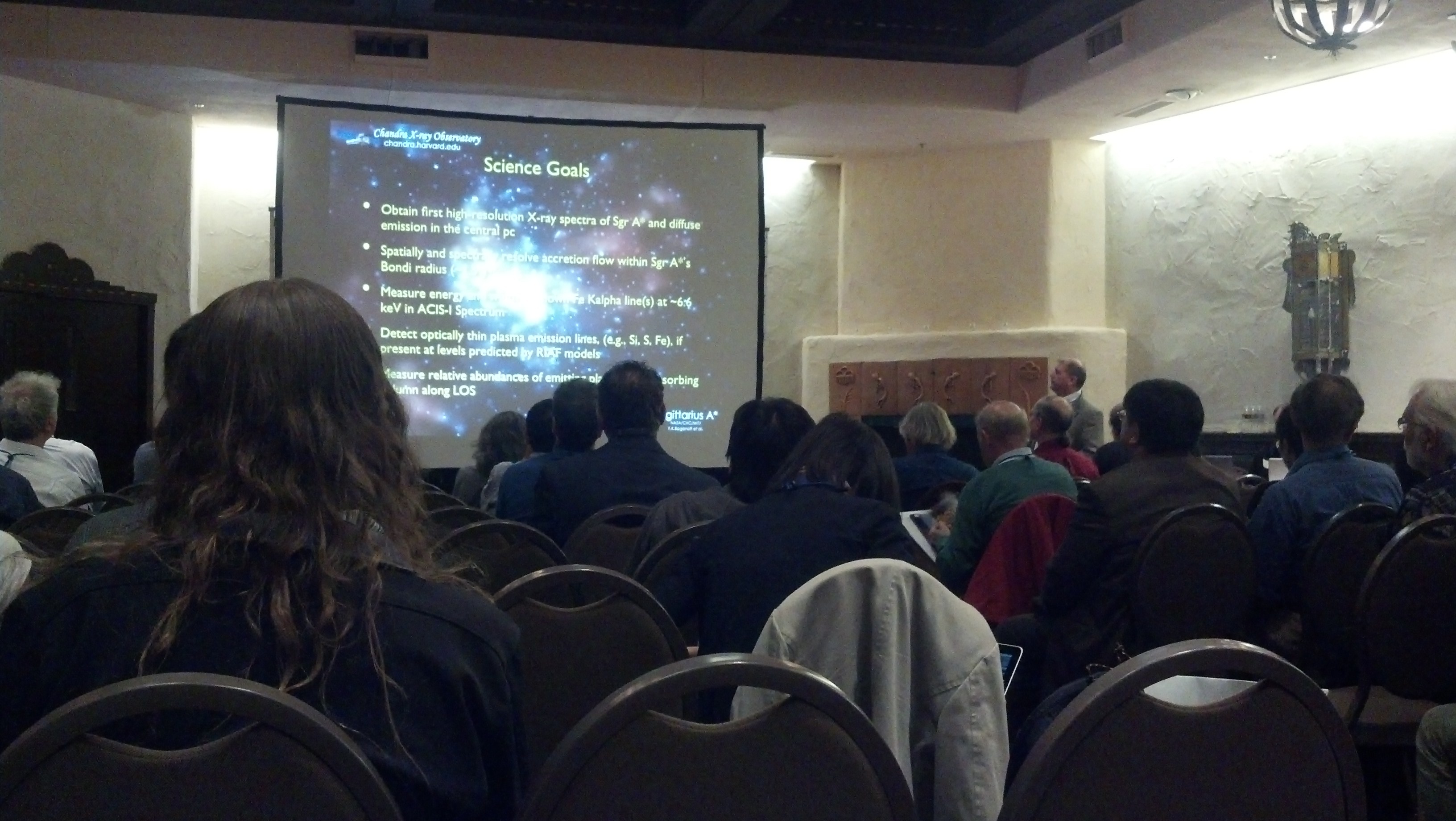
Fred Baganoff: X-ray Visionary Project: SgrA*
- High-res x-ray spectra of Sgr A* & surrounding emission
- Radio pol obs: most accreting matter doesn't reach event horizon
- 3 Ms exposure
- specific roll-angles required because Chandra has no slit
- detected 6.67 keV Helium-like Fe K-alpha + hi-res rules out 6.4 keV emission model
- What mechanism drives Sgr A* flares?
- what x-ray emission mechanism? Thermal? Compton? Synchro? etc.
- X-ray/NIR variable
- mm/radio events weaker, longer timescale, optically thick
- do mm/radio lead or lag?
- What determines flare cycle?
- What triggers flares?
- Observations
- Backgrounds are a big problem
- Details about order sorting, etc.
Questions
- Farhad: Discovered a lot of X-ray binaries. Find any sources within 1'?
- Found the old recurrent ones. Magnetar is new. No new bright ones, searching for faint ones. Vast population of faint variables.
- Q: Underlying physical mechanism still unknown. Where are we going? How do we figure it out?
- A: NuStar will help. Very narrow window; can't see optical or UV. This campaign gives more examples.
- Cornelia: Is anyone working on the diffuse? Nonthermal filament sticks out brightly
- Yes. Sgr E & F sources. Studying with NuStar team.
- Q: Can you create images with 3Ms spectra?
- A: Not much better; the grating reduces raw sensitivity.
- Q: Dismissed possibility of periodicity. Have you carefully looked? Lomb-Scargle?
- A: Lots of times with no flaring obvious. But, maybe a lot missed below the noise of the DC signal. Brightest peaks are not periodic. Peaks put into Lomb-Scargle, but not enough data for that. Will look at power spectrum though.
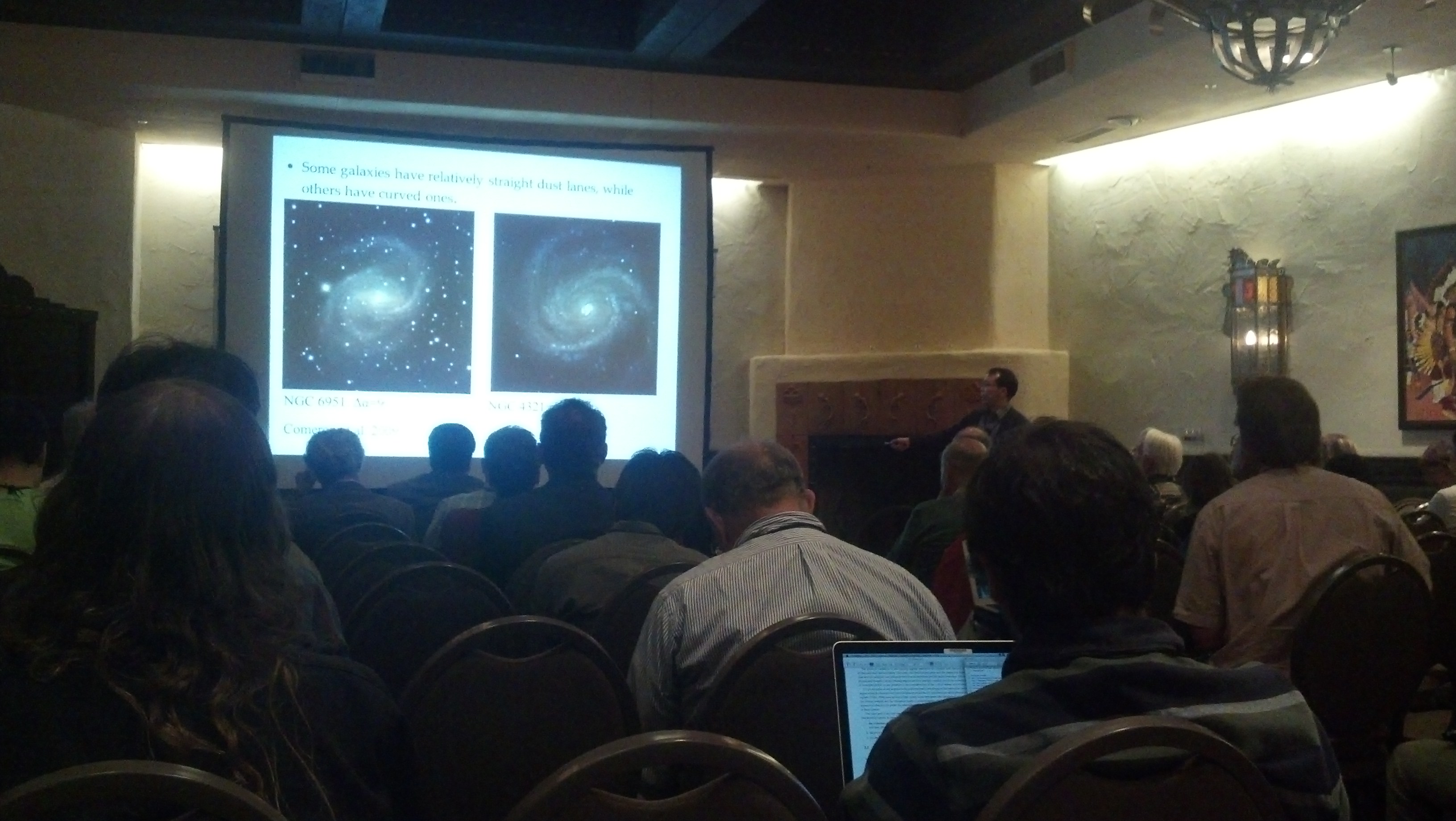
Woong-Tae Kim: Star Formation in Nuclear Rings
Nuclear Rings
- Form by resonant interactions with barred potentials + but bar torque is low near inner lindbland resonances + resonance is very long timescale
- claim that bar strength controls bar substructure
- bar potential modeled by "Ferrers Prolates"
- Q_B is the "controlling parameter" + Q_B = 0.23 yields really cool looking models
- stronger bar leads to smaller radius ring + pushes more gas inward
- range of SFR + age gradient within nuclear rings
Two models of ring SF
- popcorn model + randomly distributed + no age gradient
- pearls-on-a-string model + SF at contact point + age gradient
- age gradient <-> lower SFR
- simulation generating 10^5 msun clusters
Sim results
- presence or absence of age gradient depends on SFR + no age gradient if SFR > 1 Myr + corresponds to maximum SFR at a contact point
- prolonged SF requires prolonged feeding + HVCs (accretion of primordial gas) + ang mom dissipation by spiral arms + Galactic fountains
- If corotation radius at large R, can feed spiral arms into ring
Questions
- Q: Sims are pure hydro. Speculate on B-fields. Chuckle.
- A: Ring would be smaller
- Q: Typical velocity of gas along bar in model?
- A: 50-100 km/s
- Q: Do you mean no need for x2 orbit?
- A: no, need X2 to form ring. Formation mechanism of ring is not related to resonance.
- Q: Ring on x2 orbit?
- A: yes
- Q: is there observation evidence of age gradients in nuclear rings?
- A: Yes, Mazzuca '08 shows gradient in H-alpha EQW
- Q Farhad: Can you form the circumnuclear disk (2pc) with the same mechanism?
- A: Can't answer now. Need to run the simulation with the right size-scale
- Q: Would the bar be unstable to bending instabilities in 3D?
- A: We ran 3D, and didn't see any difference. But, with different initial conditions, may see dynamical difference..
- Q: Have you modeled where the bar meets the arm?
- A: No, couldn't do that, only treated stellar.
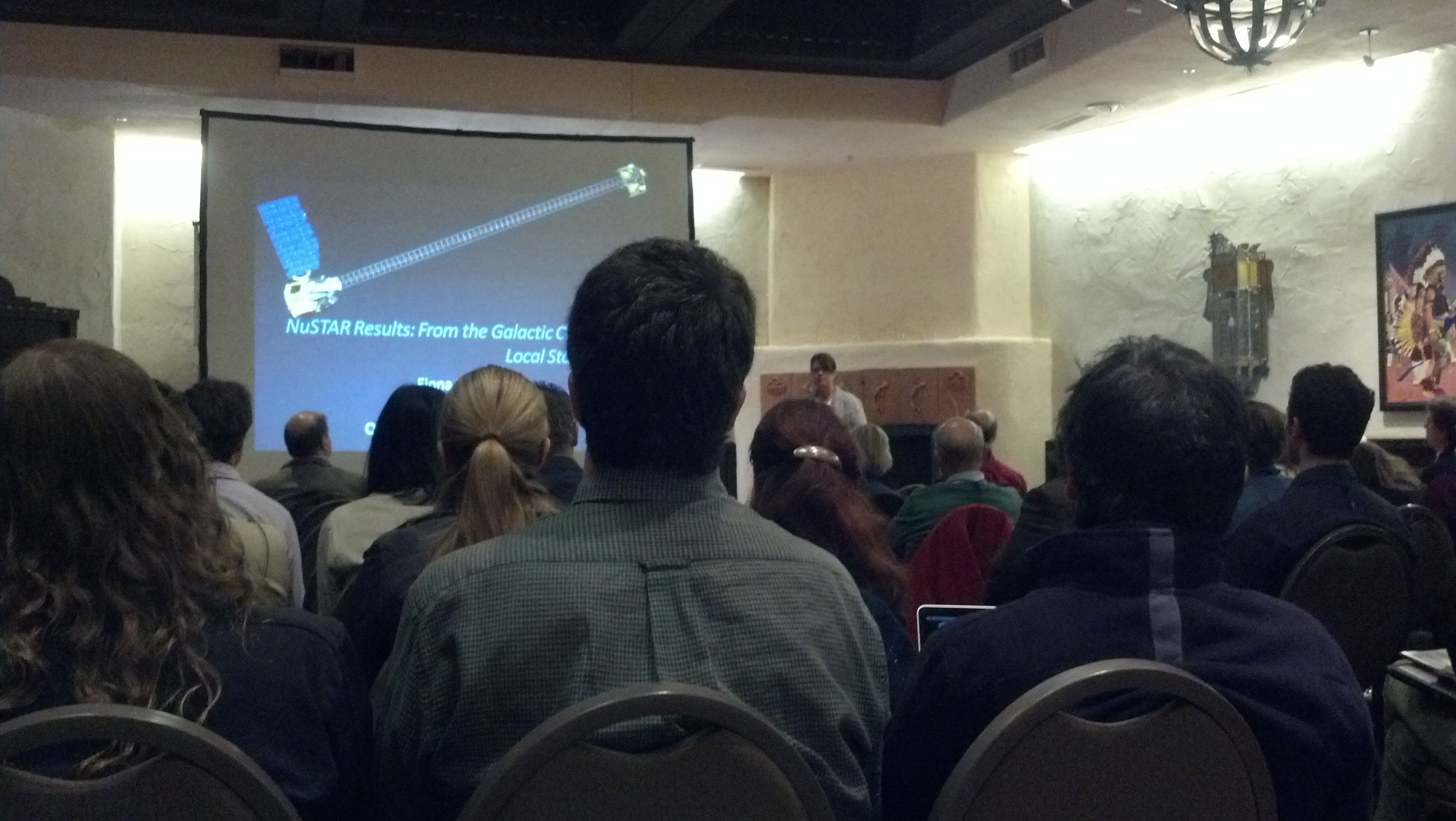
Fiona Harrison: NuSTAR Results: From the Galactic Center to Local Starbursts
- NuStar
- Explorer class
- PI-led
- Will have guest investigator program
- First focusing telescope in high-energy X-ray band
- 100x improvement in 3-79 keV
- Previous telescopes: detector was larger than collecting area of telescope
- ~18" resolution, 12.5' fov
- Our CMZ: Multicolor cmz vs INTEGRAL
- NUstar FOV = Integral resolution
- Survey Muno field (CMZ surey covering negative longitudes)
- Sgr A*
- Flares show it obviously
- ~1hr/day
- detection of flare at >10 keV
- Gamma ray pulse in Galactic Center
- enhanced X-ray emission
- pulsations detected
- 3.7 second pulsations
- 3" distant magnetar: SGR J1745-29
- Associated with disk of massive stars near Sgr A*?
- HESS J1640-465
- being observed right now
- TeV source
- possible evidence from NuStar for a pulsar
- Nearby Starburst Galaxies
- Observations coordinated with Chandra
- NGC 253, Arp 299, M82, NGC 3310, NGC 3256
- AGN may only be visible at high energies b/c of absorption at lower energies
- sampling range in mass, sfr
- NGC 253
- Lehmer et al 2013
- Where is the nucleus? Crowded core, hard to determine
- Chandra obscured X-ray source "off-center" compared to Radio
- dynamical center determined; Chandra sees one source near it + variability driven by that source + nustar spectrum by assuming all variability associated with it + classical ULX source: binary star + BH + Either IMBH or super-eddington accretion
- nuclear emission overestimated due to ULXs
- Arp 299
- Only "B" nucleus visible at high X-ray energies
- Only one nucleus currently active
Questions:
- Farhad: Will Nu-Star look at gamma-ray bubble?
- A: Two problems: 1. too extended, too much time, can't contribute much
- Is there a possibility of other magnetars not yet detected?
- A: Various types of magnetars. Undetectable in quiescence. Difficult to constrain overall population. Raises questions: unlikely by chance; do we not understand magnetar population
- What is the diffuse emission detected with INTEGRAL? In Sgr E?
- A: We don't see hard x-ray emission coincident with INTEGRAL source. Centroid of INTEGRAL source offset from diffuse emission
Susanne Aalto: Physical Conditions and Chemistry of Molecular Gas in Galactic Centers
Physical conditions & chemistry
- Astrochemistry as a diagnostic...
- 50+ molecules detected exgalactically
- CO n>10^2, HCN n>10^4
- temperature NH3, H2CO
- Only works if molecules excited by collisions
- 12CO/13CO increases towards GC because more diffuse gas [my q: integrated?]
- "Raisin Roll" view:
- Mol massin dense clumps, HI diffuse throughout
- HCO+, H3O+, HNC, HC3N, CN, SiO, H2O
- General Trends
- HNC 1-0 anticorrelated with HCN+ 1-0
- C2H ubiquitous
- "Hot Cores"
- Arp 220
- Drive outflows
- "Boring" NGC 1377 (optically) + has very deep SiO absorption + molecular outflow M~10^7 Msun + 860um optically thick core
- NGC 4418 "Ugly Duckling" galaxy + optically thick "atmosphere" dust core surrounded by molecular disk + N~10^25 cm^-2 + inner temp ~200-300K + molecular "disk" ~50K
- unclear how common optically thick cores are + can be studied with vibrationally excited molecules
- NGC 4418 + Global spectrum dominated by vibrationally excited HC3N
- Mrk231 + HCN outflow, 1000 km/s + vibrationally excited HCN in core
- vibrationally excited lines trace warped disk
- Arp 220W: amplified IR-pumped HNC
- ALMA NGC 4418 "spectral scan"
- dominated by vibrational lines
- SMA spectral scanning in Arp 220
- problematic: wide lines
- vibrational lines are the new standard
- Less obscured galaxies
- NGC 253, IC 342, Maffei 2, NGC 1068...
- same chemistry can trace outflows or star formation
- HNC, HCN, HCO+ correlated with 3mm continuum: trace SF
- HNCO, CH3OH, SiO anti-correlated with SF: probably trace outflows
- N2H+ - "warm gas" and "warm dust". Not the same in our galaxy & others
- NGC 1068
- PdBI Spirals around center
- ALMA bar + spirals + central cirumnuclear disk
- complicated chemistry towards true center
- noncircular motions
- More results:
- ALMA + ATCA towards Cen A
- NGC 1097
- HC3N in Mrk 231
- HCN in wind... extreme hcn abundance
Questions:
- Inner NGC 1068 ring - what resolution can you get with ALMA? Can you see kinematics?
- A: Yes, can see kinematics. 0.1", can do ~10x better eventually. 400 km/s
- Draw attention to MOPRA MALT-90: good comparison survey for galaxies
- Thanks
John Bally - Hi-Gal CMZ
- Summary of Hi-Gal:
- 900hrs,
- inner ±60 deg, then outer ±60 deg, then full 360 deg.
- Release scheduled late in 2013.
- 0.5 million band-merged sources
The CMZ:
- we live in a mildly barred galaxy
- NGC 1097 as an analog
- our CMZ less symmetric
Multiwave comparison:
- asymmetry: 24, 70 right; gas left
- snrs, evolved stars, nonthermal filaments, arched filaments...
The Gas:
10^7 Msun
CMZ clouds more massive, more turbulent
Cold gas to the left of Sgr B2, warmer to the right
Column density somewhat flat from l=1.5 to l=0 + "Optically thick as a brick"
Molinari "ring" - column density, some evidence from velocities + vertical oscillation = 2x circular speed + offset... + predicts Sgr B2 at tangent of ring
- velocity of Sgr B2 too slow
- Sgr B2 has significant proper motion: 80 km/s
- Molinari ring falsified: must extend to larger long
Few point sources in the Arched Filaments
- Sofue-Handa ('84) lobe:
- brightest super-bubble in galaxy
- powered by AGN or starburst?
- Warning: Lots of foreground towards CMZ. + Sco-Cen group + radio emission associated with wall of scocen
- Sgr B2 spectroscopy:
- Two temperature components in Sgr B2
- PACS sees 300K CO
Sgr C mention
- Bania's clump
- 200 km/s linewidth
- The Brick
- most extreme IRDC
- 24, 70 opaque
- HCO+ cubes
- Dust
- Are dust grains different?
- Temperature differs between gas and dust
- Questions:
- COMMENT: NGC 1068 has 100 pc molecular ring, will mention later in discussion
- Lang: Sources in arched filaments - are they aligned with filament?
- A: Yes, 50-60 in filament. SEDs look like protostars.
- Jerry (?): Note - hard to avoid conical wind from Sgr A* dynamically.
- Bally: Yes. High-latitude CO gas off-plane: entrained. Starburst likely, AGN unlikely to entrain it.
- Jay Gallagher: M82 energy density ~100x higher than in MW, driving wind out of smaller potential. Galaxy requires huge pressure change.
- Bally: Yes, wimpy nucleus
- Michael: Evidence for bar from cobe & spitzer. Is it related to gas bar?
- Bally: Related. Gas bar 20 ±3 from line of sight, but infrared stellar bar more like 45 degrees. Why offset? controversial. Generically related.
Position-Velocity Diagrams
tl;dr version: IPython notebook here, code available on github
Current state of affairs
Position-velocity diagrams with arbitrary position axes have been a common tool for studying spectra for a long time, probably because the "native" format of long-slit spectra on CCDs is effectively a position-velocity diagram.
It's becoming more common now to have data cubes (PPV) than 1D or 2D spectra. But PV diagrams still have utility. Unfortunately, there aren't very good tools to produce them.
There are plenty of tools that can slice along any of the native axes of a data cube. If you take your data cube in RA/Dec space, extracting along lines of constant RA or Dec is trivial (GAIA can do it natively, but it's easy to slice a cube in IDL or python).
However, if you wanted to slice along lines of constant GLON or GLAT, you'd have to reproject the cube to use this approach. There are nice tools that implement cube rotation: CASA has an imrebin recipe and STARLINK has a rotation tool (though I can't find it now...).
However, this approach is terribly inefficient if you want slices at multiple different angles, and it's outright awful if you want to track a filament.
An alternative approach
The alternative is to interpolate between pixels along a specified axis. This can be done very efficiently in python using scipy's map_coordinates, which by default does a cubic-spline interpolation at the specified points.
I've started to build a tool to extract position-velocity diagrams on this basis. It's fully functional, but doesn't do anything interactive just yet. pvextractor is available on github.
There is a complete example demonstrating its use here.
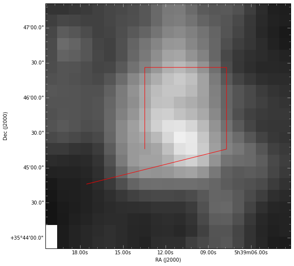
In short, though, it allows you to describe paths like this:
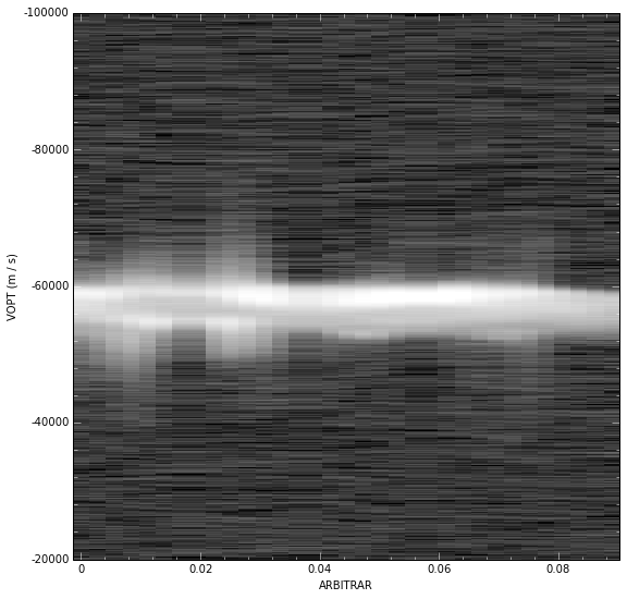
and extract them into position-velocity diagrams like this:
Blogging from IPython
[ Notebook Form of this post ]
There have been many other posts about blogging in ipython, but they all included more overhead than I really wanted to deal with.
Instead, I've gone directly to the source and used nbconvert in ipython 2.0 to convert my notebooks to rst, then put them through pelican.
This post outlines my workflow.
First, and most inconvenient, it is necessary to head any blog post with metadata. I don't have any convenient workflow to deal with that, I just write it in by hand in a raw text box (ctrl-m, t) as you can see above. Daniel Rodriguez took a different approach using the ipython metadata directly and an ipython plugin, but I didn't want to have to worry about installing plugins and I am definitely worried about breaking notebooks by messing with the metadata as the ipy devs give some fairly strict warnings.
Next, the ipynb -> rst step is fairly straightforward. I modified the rst template because I don't want to see the In[#]: and Out[#]: prefixes around my code. I also use .. code-block:: rather than .. code::.
This very simple function below makes sure that my local rst.tbl file is seen before ipython's. Their templates are in IPython/nbconvert/templates. Note that you could normally use Jinja2 templating and "Extend" their template, but I wanted to remove rather than extend.
[ Source ]
from IPython.nbconvert.exporters import RSTExporter def export(nbname, outfilename=None): exportRST = RSTExporter() # exclude default paths exportRST.template_path = ['.','/Users/adam/repos/blog'] (body,resources) = exportRST.from_filename(nbname) if outfilename is None: outfilename = nbname.replace("ipynb","rst") with open(outfilename,'w') as f: f.write(body) return body,resources
I then run the script from the command line: ~/virtual-ipydev/bin/ipython ./nbconverter.py content/GenerateCVExample.ipynb
I'm using a virtual environment with ipython 2 installed because I'm not yet ready to make the jump to the dev version of ipython (though these days, with Travis and Jenkins around, it's probably safe to assume the dev version won't break anything).
With this rst file generated, the only remaining step is pelican, which only requires a make github command in the blog directory. Installing & setting up pelican is reasonably easy, but not the topic of this post.
I've made my own custom pelican theme, so I generally need to update the theme before building:
pelican-themes --upgrade /Users/adam/repos/pelican-themes/mine && make github
Generating a CV using the ADS Labs API
At .astronomy this past week, the keynote speaker was Alberto Accomazzi, introducing ADS Labs and ADS 2.0, which are really quite impressive.
I was inspired to use ADS Labs to help me auto-generate a nicely formatted CV for myself. I used Andy Casey's ADS-python as a starting point: he introduces a useful convention of storing your ADS API Key:
import os def get_dev_key(): """ A convenience function for accessing a system-wide ADS Developer's Key """ ads_dev_key_filename = os.path.abspath(os.path.expanduser('~/.ads/dev_key')) if os.path.exists(ads_dev_key_filename): with open(ads_dev_key_filename, 'r') as fp: dev_key = fp.readline().rstrip() return dev_key if 'ADS_DEV_KEY' in os.environ: return os.environ['ADS_DEV_KEY'] raise IOError("no ADS API key found in ~/.ads/dev_key")
We'll use requests to send the request to ADS, then json to parse the data.
import requests import json
We then query the database using a keyword query (parameter q) specifying the author. Other required parameters are the API key (dev_key) and a filter to select only astronomy articles. The maximum number of rows returned in the API is 200 right now, which I have set (the default is 10 or 20).
response = requests.post('http://adslabs.org/adsabs/api/search/', params={'q':'author:ginsburg, a', 'dev_key':get_dev_key(), 'rows':200, 'filter':'database:astronomy'})
J = response.json() J.keys()
[u'meta', u'results']
The JSON 'meta' key is just metadata about the query, include the number of matches and execution time.
J['meta']
{u'api-version': u'0.1', u'count': 54, u'hits': 54, u'qtime': 7, u'query': u'author:ginsburg, a'}
The 'results' key includes what we're actually interested in, under another key 'docs'.
J['results'].keys()
[u'docs']
datalist = J['results']['docs'] type(datalist), len(datalist)
(list, 54)
datalist is a list of the retrieved bibliographic entries.
datalist[0].keys()
[u'bibcode', u'keyword', u'pubdate', u'bibstem', u'property', u'aff', u'author', u'citation_count', u'pub', u'page', u'volume', u'database', u'doi', u'year', u'abstract', u'title', u'identifier', u'issue', u'id']
At this point, most of the remaining work is building up a nicely formatted output. We'll start with a web-specific example, using HTML unordered lists.
In this example, we'll make a list item that creates a hyperlink for the author names and uses a reasonably standard bibliographic format:
Authors Month, Year, Journal Title
fmt = (u' ' u'<li><a class="norm" href="http://adsabs.harvard.edu/abs/{adsbibid}">{creator}</a>' u' {month}, <b>{year}</b> {journal}\n' u' <br> {titlestring}')
We need to do a little data wrangling to get the individual JSON entries into the appropriate format:
def wrangle(data, authorname='Ginsburg'): """ Create new fields from the input data to insert into the format string """ data['month'] = data['pubdate'][5:7] # Generally, the last identifier is the published version, # while the first is an arXiv identifier # (data['identifier'] is a list) data['adsbibid'] = data['identifier'][-1] # data['title'] & ['pub'] are also lists data['titlestring'] = data['title'][0] data['journal'] = data['bibstem'][0] # This trick bolds my name in the list of authors data['authors'] = ['<b>{}</b>'.format(x) if authorname in x else x for x in data['author']] # Separate names by semicolons data['creator'] = u"; ".join(data['authors']) return data
The return from wrangle is a dict with new keys that match the keywords in the format string. The python string.format method will nicely ignore any extra keywords that we're uninterested in.
fmt.format(**wrangle(datalist[0]))
u' <li><a class="norm" href="http://adsabs.harvard.edu/abs/2013ApJ...773..102F">Fallscheer, C.; Reid, M. A.; Di Francesco, J.; Martin, P. G.; Hill, T.; Hennemann, M.; Nguyen-Luong, Q.; Motte, F.; Men'shchikov, A.; Andrxe9, Ph.; Ward-Thompson, D.; Griffin, M.; Kirk, J.; Konyves, V.; Rygl, K. L. J.; Sadavoy, S.; Sauvage, M.; Schneider, N.; Anderson, L. D.; Benedettini, M.; Bernard, J. -P.; Bontemps, S.; <b>Ginsburg, A.</b>; Molinari, S.; Polychroni, D.; Rivera-Ingraham, A.; Roussel, H.; Testi, L.; White, G.; Williams, J. P.; Wilson, C. D.; Wong, M.; Zavagno, A.</a> 08, <b>2013</b> ApJn <br> Herschel Reveals Massive Cold Clumps in NGCxa07538'
Now to show it in the notebook...
import IPython.display IPython.display.HTML(fmt.format(**wrangle(datalist[0])))
You can make a complete bibliography by looping over a few entries. The ordered list (<ol>) tag makes a numbered list.
html = "<ol>" + "\n".join(fmt.format(**wrangle(datalist[ii])) for ii in xrange(3)) + "</ol>" IPython.display.HTML(html)
If you want to make sure you only include refereed articles, use the 'property' tag.
print ['REFEREED' in d['property'] for d in datalist]
[True, False, True, False, False, False, True, True, False, False, False, False, True, True, True, False, False, True, True, False, False, True, True, True, False, False, False, False, True, False, False, True, True, True, True, True, True, False, False, False, False, False, False, True, True, False, False, False, False, False, True, False, False, True]
And don't forget that you can also include the citation count:
print "\n".join(["{} {}: {}".format(d['author'][0],d['year'],d['citation_count']) for d in datalist if 'citation_count' in d and 'REFEREED' in d['property']])
Fallscheer, C. 2013: 0 Ellsworth-Bowers, Timothy P. 2013: 2 Smith, Nathan 2013: 0 Harvey, Paul M. 2013: 2 Bressert, E. 2012: 10 Ginsburg, A. 2012: 11 Bally, John 2012: 0 Ginsburg, Adam 2011: 5 Battersby, C. 2011: 22 Schlingman, Wayne M. 2011: 17 Ginsburg, Adam 2011: 6 van Aarle, E. 2011: 12 Aguirre, James E. 2011: 72 Bally, John 2010: 36 Battersby, Cara 2010: 30 Yan, Chi-Hung 2010: 5 Bally, J. 2010: 20 Dunham, Miranda K. 2010: 27 Rosolowsky, Erik 2010: 80 Ginsburg, Adam G. 2009: 10 Rubin, D. 2009: 23 van de Steene, G. C. 2008: 4 Golitsyn, G. S. 1985: 4
Wishlist
There are a few other features that would be nice to add to the CV, but some are not yet well-supported.
- You can get the full name, but right now not the short name ('bibstem'), of the journal
- The bibtex entry is important for generating tex versions of CVs. Currently, it is not possible to completely reproduce one, largely because of point #1.
However, the ADS folks will certainly change this soon. You can find out if they have by querying their API settings. If the query below returns "True", then you can access the bibstem.
UPDATE 9/23/2013: Jay Luker @ADS added 'bibstem' to the allowed return entries
permissions_response = requests.post('http://adslabs.org/adsabs/api/settings/',params={'dev_key':get_dev_key()}) permissions = permissions_response.json() 'bibstem' in permissions['allowed_fields']
True
In the meantime, you can get most of the way there. We'll create "Article" entries for any articles or eprints and ignore abstracts (e.g., conference abstracts). I don't have any books, but for others that might be useful.
The approach we'll use is also a good way to reject unwanted articles in the HTML bibliography above.
bibfmt = u"""@article{{{tagname}, abstract={{{abstract}}}, author={{{bibtexauthors}}}, month={{{month}}}, pages={{{page}}}, title={{{titlestring}}}, year={{{year}}}, volume={{{volume}}}, journal={{\\{lowercasejournal}}} }}"""
Of course, it's necessary to wrangle the data again for the appropriate author list formatting for bibtex:
def wrangleauthors(authorlist): """ Fit the author list into a bibtex-friendly format. Not the cleanest hack, since we need to allow for single-name authors (e.g., astropy collaboration, Planck collaboration, etc.) The triple braces are needed because TeX uses them""" splita = [[b.strip() for b in a.split(",")] for a in authorlist] bracketed = [u'{{{}}}, {}'.format(a[0], a[1].replace(" ","~")) if len(a) > 1 else u'{{{}}}'.format(a[0]) for a in splita] return u" and ".join(bracketed)
wrangleauthors(datalist[0]['author'])
u"{Fallscheer}, C. and {Reid}, M.~A. and {Di Francesco}, J. and {Martin}, P.~G. and {Hill}, T. and {Hennemann}, M. and {Nguyen-Luong}, Q. and {Motte}, F. and {Men'shchikov}, A. and {Andrxe9}, Ph. and {Ward-Thompson}, D. and {Griffin}, M. and {Kirk}, J. and {Konyves}, V. and {Rygl}, K.~L.~J. and {Sadavoy}, S. and {Sauvage}, M. and {Schneider}, N. and {Anderson}, L.~D. and {Benedettini}, M. and {Bernard}, J.~-P. and {Bontemps}, S. and {Ginsburg}, A. and {Molinari}, S. and {Polychroni}, D. and {Rivera-Ingraham}, A. and {Roussel}, H. and {Testi}, L. and {White}, G. and {Williams}, J.~P. and {Wilson}, C.~D. and {Wong}, M. and {Zavagno}, A."
Now we can start looping through, performing checks for article status, and making bibentries. We'll use python's dateutils.parse to turn month numbers into names
import dateutil.parser
for d in datalist: d['bibtexauthors'] = wrangleauthors(d['author']) # pubdates don't include days, and sometimes don't include months, # so we have to be careful d['month'] = (dateutil.parser.parse(d['pubdate'][:-3]).strftime("%B") if d['pubdate'][5:7] != '00' else "") # To make the standard macros, e.g. \apj, \aa d['lowercasejournal'] = d['bibstem'][0].lower() # list -> string d['titlestring'] = d['title'][0] # need to make sure there is something to put in the volume field d['volume'] = d['volume'] if 'volume' in d else '' # tagname is [First author's last name][year] d['tagname'] = d['author'][0].split()[0].strip(",") + d['year']
bibdata = "" for d in datalist: if 'ARTICLE' in d['property'] or 'EPRINT' in d['property']: bibdata += bibfmt.format(**d) + "\n\n"
Now this data can be saved to a bibliography file and parsed by LaTeX.
import codecs # for writing unicode with codecs.open('mypapers.bib','w',encoding='utf8') as f: f.write(bibdata)
Future work:
- Verify the bibtex
- Generate the CV LaTeX and compile it
My favorite Splatalogue queries
I tend to be most interested in low-energy molecular lines: CO, NH3, and H2CO being the main candidates.
Note: Splatalogue has made some recent changes to their returned tables, partly per my recommendations. The code below has been update to reflect these changes.
>>> from astropy import units as u >>> from astroquery.splatalogue import Splatalogue >>> S = Splatalogue(energy_max=500, ... energy_type='eu_k',energy_levels=['el4'], ... line_strengths=['ls4'], ... only_NRAO_recommended=True,noHFS=True) >>> def trimmed_query(*args,**kwargs): ... columns = ('Species','Chemical Name','Resolved QNs','Freq-GHz', ... 'Meas Freq-GHz','Log<sub>10</sub> (A<sub>ij</sub>)', ... 'E_U (K)') ... table = S.query_lines(*args, **kwargs)[columns] ... table.rename_column('Log<sub>10</sub> (A<sub>ij</sub>)','log10(Aij)') ... table.rename_column('E_U (K)','EU_K') ... table.rename_column('Resolved QNs','QNs') ... table.sort('EU_K') ... return table >>> trimmed_query(1*u.GHz,30*u.GHz, ... chemical_name='(H2.*Formaldehyde)|( HDCO )', ... energy_max=50).pprint() Species Chemical Name QNs Freq-GHz Meas Freq-GHz log10(Aij) EU_K ------- ------------- ------------- -------- ------------- ---------- -------- HDCO Formaldehyde 1(1,0)-1(1,1) -- 5.34614 -8.31616 11.18287 H2C18O Formaldehyde 1(1,0)-1(1,1) 4.3888 4.3888 -8.22052 15.30187 H213CO Formaldehyde 1(1,0)-1(1,1) -- 4.59309 -8.51332 15.34693 H2CO Formaldehyde 1(1,0)-1(1,1) 4.82966 -- -8.44801 15.39497 HDCO Formaldehyde 2(1,1)-2(1,2) -- 16.03787 -7.36194 17.62746 H2C18O Formaldehyde 2(1,1)-2(1,2) 13.16596 13.16596 -6.86839 22.17455 H213CO Formaldehyde 2(1,1)-2(1,2) -- 13.7788 -7.55919 22.38424 H2CO Formaldehyde 2(1,1)-2(1,2) 14.48848 -- -7.49383 22.61771 H2C18O Formaldehyde 3(1,2)-3(1,3) 26.33012 26.33014 -6.03008 32.48204 H213CO Formaldehyde 3(1,2)-3(1,3) -- 27.55567 -6.95712 32.9381 H2CO Formaldehyde 3(1,2)-3(1,3) -- 28.9748 -6.89179 33.44949 >>> trimmed_query(100*u.GHz,400*u.GHz, ... chemical_name='Carbon Monoxide', ... energy_max=50).pprint() Species Chemical Name QNs Freq-GHz Meas Freq-GHz log10(Aij) EU_K ------- --------------- ----- --------- ------------- ---------- -------- C18O Carbon Monoxide 1-0 109.78218 109.78218 -7.20058 5.26868 13COv=0 Carbon Monoxide 1-0 110.20135 -- -7.49946 5.2888 C17O Carbon Monoxide J=1-0 112.35928 112.35928 -7.17404 5.39236 COv=0 Carbon Monoxide 1-0 115.2712 115.2712 -7.14236 5.53211 C18O Carbon Monoxide 2-1 219.56036 219.56036 -6.21833 15.80595 13COv=0 Carbon Monoxide 2-1 220.39868 -- -6.51752 15.86618 C17O Carbon Monoxide J=2-1 224.71437 224.71439 -6.19179 16.17703 COv=0 Carbon Monoxide 2-1 230.538 230.538 -6.16011 16.59608 C18O Carbon Monoxide 3-2 329.33055 329.33055 -5.66014 31.6116 13COv=0 Carbon Monoxide 3-2 330.58797 -- -5.95976 31.73179 C17O Carbon Monoxide J=3-2 337.0611 337.06113 -5.6336 32.3538 COv=0 Carbon Monoxide 3-2 345.79599 345.79599 -5.60192 33.19169 >>> trimmed_query(1*u.MHz,2*u.GHz, ... chemical_name=' H2CO .*Formaldehyde',energy_max=75, ... energy_type='eu_k').pprint() Species Chemical Name QNs Freq-GHz Meas Freq-GHz log10(Aij) EU_K ------- ------------- ------------- -------- ------------- ---------- -------- H2CO Formaldehyde 2(2,0)-2(2,1) -- 0.07114 -13.81846 57.612 H2CO Formaldehyde 3(2,1)-3(2,2) -- 0.35557 -12.02319 68.11082 >>> trimmed_query(20*u.MHz,25*u.GHz,chemical_name=' NH3 ').pprint() Species Chemical Name QNs Freq-GHz Meas Freq-GHz log10(Aij) EU_K ------- ------------- -------------- -------- ------------- ---------- --------- NH3v=0 Ammonia 1(1)0a-1(1)0s 23.69447 23.6945 -6.43769 24.40492 NH3v=0 Ammonia 2(2)0a-2(2)0s 23.7226 23.72263 -6.31125 65.5867 NH3v=0 Ammonia 2(1)0a-2(1)0s 23.09885 23.09881 -6.94808 81.5904 NH3v=0 Ammonia 3(3)0a-3(-3)0s 23.87008 23.87013 -6.25203 124.68113 NH3v=0 Ammonia 3(2)0a-3(2)0s 22.83422 22.83418 -6.662 151.33353 NH3v=0 Ammonia 3(1)0a-3(1)0s 22.23456 22.2345 -7.29889 167.29666 NH3v=0 Ammonia 4(4)0a-4(4)0s 24.13935 24.13942 -6.20938 201.67106 NH3v=0 Ammonia 4(3)0a-4(-3)0s 22.68835 22.68831 -6.54002 238.96192 NH3v=0 Ammonia 4(2)0a-4(2)0s 21.70341 21.70336 -6.95001 265.52612 NH3v=0 Ammonia 4(1)0a-4(1)0s 21.13434 21.13431 -7.58659 281.43749 NH3v=0 Ammonia 5(5)0a-5(5)0s 24.53292 24.53299 -6.1706 296.53357 NH3v=0 Ammonia 5(4)0a-5(4)0s 22.65307 22.65302 -6.46829 344.46226 NH3v=0 Ammonia 5(3)0a-5(-3)0s 21.28532 21.28528 -6.79928 381.6003 NH3v=0 Ammonia 5(2)0a-5(2)0s 20.37145 20.37145 -7.20859 408.05568 NH3v=0 Ammonia 5(1)0a-5(1)0s 19.83833 19.83835 -7.84539 423.90259 NH3v=0 Ammonia 6(5)0a-6(5)0s 22.73249 22.73243 -6.41603 467.80451