A few recent projects (ALMA W51 and ALMA Sgr B2) have raised the question: How do we interpret unresolved millimeter sources?
In the two linked works, I concluded that most of the 1mm and 3mm point sources we detected with ALMA at D>5 kpc are protostars with dust envelopes - i.e., they are "Class 0/I"-like sources, but they are generally more luminous (and therefore more massive) than their local analogs.
One of the appeals of the dust continuum, the wavelength range from about 0.5 to 2 mm, for studying star formation is that we usually assume that the source brightness is proportional to the source mass. For optically thin dust, this assumption is pretty good. The (systematic, unmeasurable) uncertainty is, to first order, just the uncertainty in the dust temperature.
However, protostellar cores - dust cores that contain a YSO or any luminous object (whether the luminosity is nuclear or gravitational in nature doesn't matter) - violate those assumptions. First, the dust is not isothermal, so the emission is weighted toward the hotter dust that represents less of the total mass. Second, the dust is not necessarily optically thin - a centrally concentrated source is likely to have a significant optical depth, particularly at the shorter wavelengths. Third, once the optically thin assumption is broken, the source geometry matters; there may be some axes along which the source is substantially brighter.
The ALMA-IMF program, which I am co-leading with Frederique Motte, Patricio Sanhueza, and Fabien Louvet, has the broad goal of understanding the formation of the IMF in the Galaxy. In practice, we will measure some form of 1 mm luminosity function. In the long term, we may be able to obtain some additional constraints on the internal temperature structures of the sources. The imminence of this large data set motivates the development of a general systematic analysis tool for assessing the implications of the mm luminosity function on the underlying mass function.
In the related Protostellar Mass Functions post, I implemented the protostellar mass functions described by McKee and Offner. These functions provide the mapping between a stellar mass function and a protostellar mass function given some assumed accretion history. The assumed accretion histories for the stars are very simple (in reality, accretion is probably quite stochastic), but that's fine since it provides something testable.
I've then tried to follow up by implementing the next step toward producing something comparable to observables as defined in Offner and McKee, but unfortunately this is a good deal more challenging. We need a means to map a protostellar mass to a luminosity, and there is no simple one-to-one function to do this.
Protostellar Evolution Models
Several authors have described protostellar evolution models. They mostly refer back to Palla & Stahler I and II. The Offner & McKee model is based on Tan & McKee 2004. There is a similar model by Hosokawa & Omukai, who have shown that high-mass stars can have substantially varying structures (radii -> luminosities) depending on their accretion rates. Mikhail Klassen implemented the Offner+ 2009 protostellar evolution models in fortran in this paper, with only slight differences assumed in the polytropic parameters and the accretion luminosity (Offner+ assumed 25% of the accretion energy is lost to wind and treated the disk and star accretion luminosity separately, according to Klassen+ 2012).
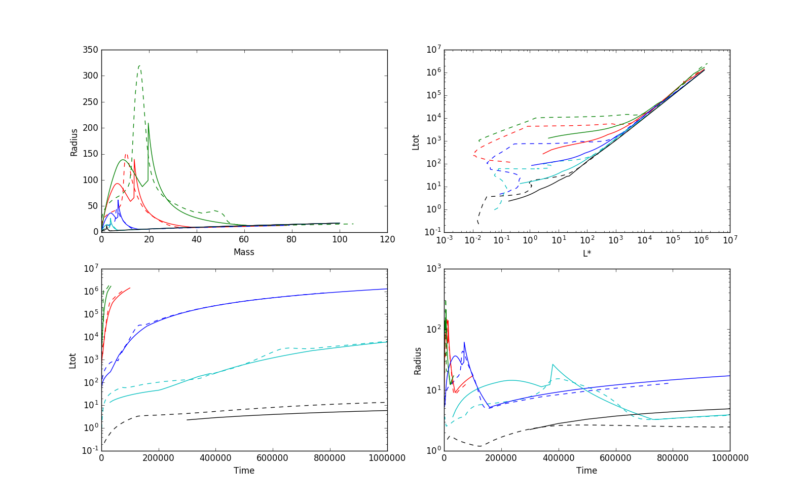
The Klassen implementation is the best immediately available to me. Both they and Offner and McKee compared their results to Hosokawa & Omukai, considering the latter to be more accurate, and found "good" agreement (<2x disagreement) in the radius as a function of mass. The same comparison is shown below; these figures match Klassen+ 2012 Figures 1 and 2 (though I don't plot exactly the same things).
At least in priniple, these tools give us a mechanism to determine L(M, M_f), the luminosity as a function of the current mass and the final mass of a star. Alternatively, that can be written as L(t, M_f), the luminosity as a function of time and final mass. However, there is at least one major practical concern: the protostellar evolution models have the free variable mdot, not M_f, so in order to use these models, we need to populate a 'fully sampled' L(M, M_f) table. Offner et al computed such a table, but then used an approximation for R(M) - the stellar radius as a function of its mass - for their calculations.
Following Offner, though, the accretion histories are not constant. Instead, they use a variety of accretion histories: isothermal sphere, turbulent core, and competitive accretion. To compute the L(M, M_f) tables, we need to run a modified version of the Klassen code with a variable accretion history.
The isothermal sphere case is actually a constant accretion rate, so that one is pretty easy. The turbulent core and competitive accretion models have an accretion rate that depends on time or mass.
Turbulent Core Protostellar Evolution
I've implemented the turbulent core accretion history in my fork of Mikhail Klassen's repository. The modification is fairly straightforward: the accretion rate is set at each timestep according to Equation 23 of McKee and Offner using the numerical constants they computed. Then, if the stellar mass has reached (or exceeds) the target stellar mass, set the accretion rate to zero. The stellar evolution code can then proceed with no further accretion.
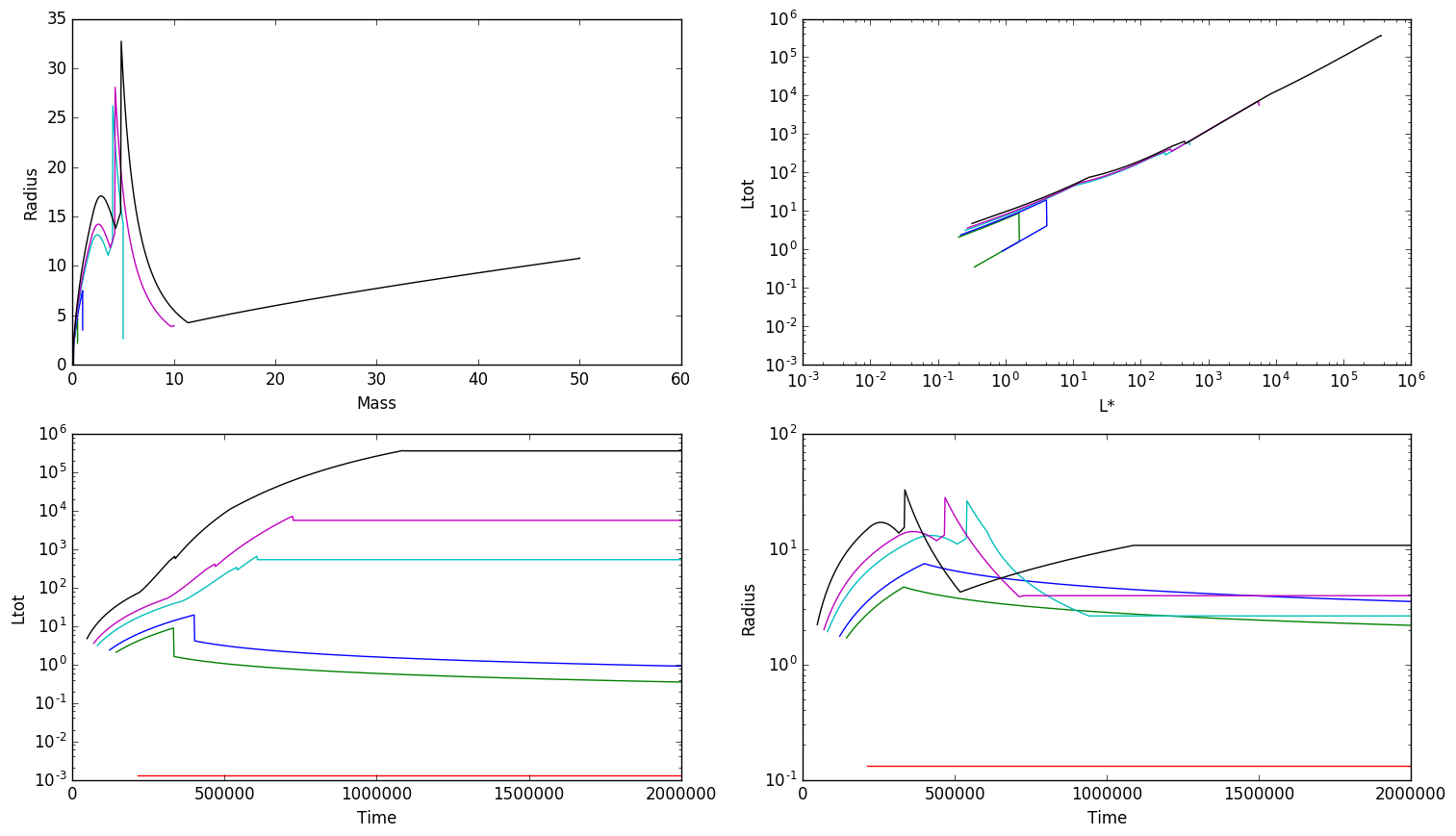
I've run this using the default initial conditions, a clump surface density $Sigma_{cl} = 0.1$ g cm$^{-2}$. The results are in the next figure: nearly all of the interesting evolution happens before the stars reach 10 Msun. The accretion luminosity is almost always subdominant, at least once anything reaches 10 Lsun. The most massive star seems to shrink below its main sequence size prior to reaching the main sequence, which is a little weird. I'm not sure if I trust that.
Further exploration of accretion history parameter space is future work. I now at least know how to set up the basic models and assemble lookup tables for L(mf,t).
Protostellar SED Models
The next step in computing a millimeter luminosity distribution is to convert from stellar luminosity to the reprocessed flux at a given wavelength. This step has an enormous number of free parameters, since the surrounding structure may include both a disk and a core whose shapes will both vary.
There are two large grids of radiative transfer models that have been computed for this purpose. The Robitaille grid is complete and open, and it should cover all stellar masses. The Zhang+ 2017 grid is not yet available, but it may be more self-consistent.
I plan to use the protostellar evolutionary model parameters, i.e., the radius and luminosity, to select models from this grid. However, the Robitaille grid uses surface temperature and radius, not luminosity and radius. So we either need to compute the stellar luminosity in the Robitaille models assuming the stars are perfect blackbodies, then use the stellar luminosity to select from that grid, or we need to compute the stellar surface temperature from the evolutionary model.
Since the Robitaille models cover a large number of parameters, but do so in a fairly sparse grid, it is not trivial to map from radius+luminosity to the models. For example, for a $2-3x10^5$ Lsun star with radius 40-50 Rsun, there are 860 models in the spubhmi grid, most of which lack flux measurements in many apertures.
Example Model Selection
For this example, I'm looking at an mf=10 Msun star at t=0.58 Myr, at which point it has m=6.5 Msun. Its radius at this time is 9.0 Rsun and stellar luminosity 1300 Lsun. This is the line of output from the Klassen model:
            Time        Stellar_Mass      Accretion_Rate      Stellar_Radius    Polytropic_Index      Deuterium_Mass       Intrinsic_Lum    Total_Luminosity    Stage
0.1842924478E+14    0.1300261603E+35    0.1404188516E+22    0.6278790980E+12    0.3000000000E+01    0.0000000000E+00    0.5084830934E+37    0.6525577133E+37        4
I select models within 5% of this one's radius and luminosity:
lum = (0.5084830934E+37*u.erg/u.s).to(u.L_sun)
rad = (0.6278790980E+12*u.cm).to(u.R_sun)
selpars = pars[(pars['Luminosity'] > lum.value*0.95) & (pars['Luminosity'] < lum.value*1.05) & (pars['star.radius']>rad.value*0.95) & (pars['star.radius']<rad.value*1.05)]
My first attempt at this, with the spubhmi model, resulted in one that has no flux in small (4000 AU) aperture, which I don't yet know how to interpret - it is certainly possible for such a source, with a non-negligible envelope, to exist, and it would certainly produce some flux.
More lenient parameters are needed:
lum = (0.5084830934E+37*u.erg/u.s).to(u.L_sun)
rad = (0.6278790980E+12*u.cm).to(u.R_sun)
apnum = np.argmin(np.abs(seds.apertures - 2000*u.au))
wav = (95*u.GHz).to(u.mm, u.spectral())
wavnum = np.argmin(np.abs(seds.wav - wav))
ok = np.isfinite(seds.val[:,wavnum,apnum])
selpars = pars[(pars['Luminosity'] > lum.value*0.9) & (pars['Luminosity'] < lum.value*1.10) & (pars['star.radius']>rad.value*0.9) & (pars['star.radius']<rad.value*1.10) & ok]
This one at least results in some hits. There are three models with fluxes (at Sgr B2, in a 2000 AU radius aperture, at 95 GHz) of 15-25, 155-170, and 55-60 mJy. To build a model cluster, we would randomly select one of these models. Robitaille notes, however, that some of the models are nonphysical; at the moment, we have no way to assess that, so we have to do the selection blindly. The brightest model has a denser envelope and more massive disk.
We can use this to make a model cluster, but this is a pretty discouraging first model given my previous work; this is presently a low-luminosity source that is surprisingly intense at 3mm.
Full Workflow
We first create a cluster by sampling from a stellar initial mass function. This part is straightforward, at least.
Then, for each source, we 'rewind' to a specific time and select model parameters from the protostellar evolution models described above. The 'rewind' could be from the point at which the stars reach "stage 5", main sequence, or we could select some other criteria.
Finally, we sample from the Robitaille parameters. For this first example, we just randomly select from some parameters that are within 5-10% of the target parameters. In the longer term, we'll want to be much more accurate and find a way to interpolate the Robitaille models onto a "fully sampled" grid of the parameter space we're interested in. The Zhang models are probably better to use once they become available since they may have accretion histories consistent with those used for the evolutionary model.
Final comments
For the next post, I hope to actually generate some clusters and see what sorts of uncertainties we're dealing with. The above examples suggest they could be truly extreme, and perhaps that the Robitaille models will be inadequate for this purpose. We'll see.