The stellar initial mass function is important for a wide variety of astronomical topics, and I'm interested in studying its formation. The protostellar mass function, by contrast, is much less well-studied, but understanding it can provide important insights into the formation of the IMF. In particular, we assume both for simplicity and because of a lack of contrary evidence, that the IMF is uniform in time in space. In other words, given that a star is going to form at some point, it has a likelihood to become a star of a given mass described exclusively by the IMF. While this assertion is entirely absurd - if you are "about to form" a star in a blob of gas that only has 0.1 Msun in a 1 pc radius, it certainly cannot form a 100 Msun star - it remains consistent with nearly all observations and is therefore used in this time- and space-invariant form.
It is likely that new studies of stellar populations, e.g., GAIA's observations of a huge population of stars with well-determined distances (and therefore luminosities), will reveal some variations in the IMF. However, many studies based on evolved stellar populations are subject to ambiguities in the initial conditions. So, it is still quite useful to study those initial conditions directly.
There has not been a huge amount of work on protostellar mass functions. McKee and Offner defined the PMF as the distribution of masses of protostellar sources that would produce a given IMF. Their PMFs are therefore strongly dependent on the underlying IMF assumed.
I have implemented the mass functions they defined in this code. The code is generalized such that you can input other mass functions. McKee & Offner only used the Chabrier 2005 mass function; I include the Kroupa 2001 mass function as well for comparison
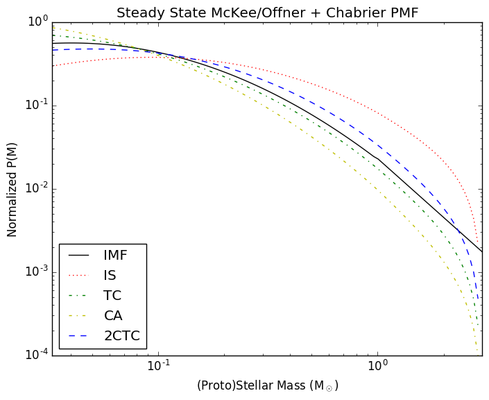
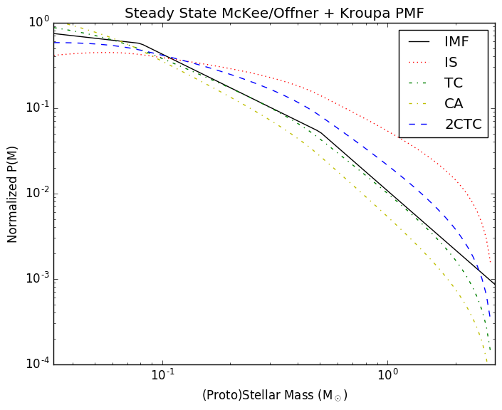
The comparison between the Chabrier and Kroupa mass functions is shown above. Note that these are somewhat deceptive plots, since they show P(M) vs log(M). The plot shows the most likely individual masses by number, but the plots are actually quite squished to the left in linear space, such that the most common range of stars (the integral of both functions) is closer to the same (~0.2-0.3 Msun). The more commonly shown version of these plots is the integral form, which has a positive power-law slope in the lowest bin in the Kroupa MF, showing the usual peak at 0.3 Msun. This version of the functions is nontrivial to compute, especially for the modified PMFs.
The mass-weighted versions of these may be more familiar, and they are more similar to the P(log M) version used in McKee and Offner and Chabrier 2005:
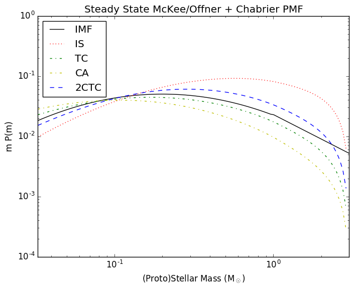
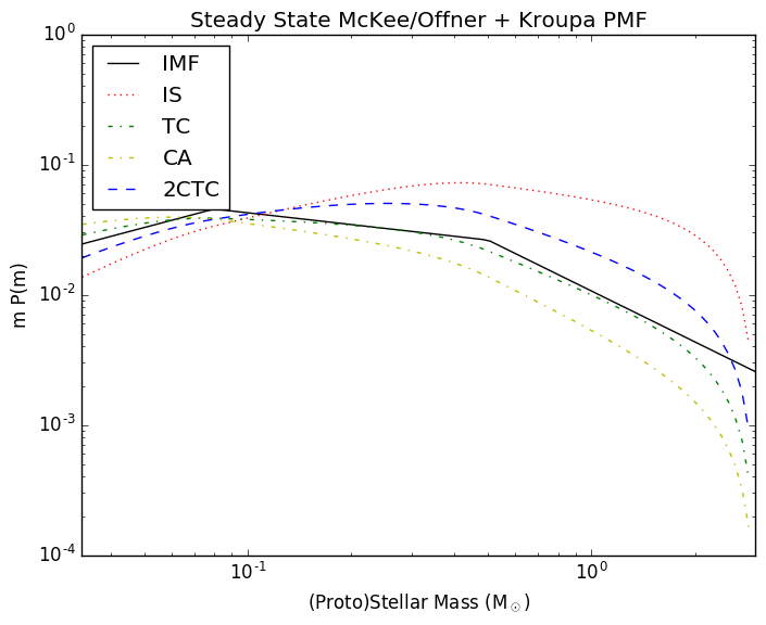
The Chabrier version is a near-perfect match to Figure 3 of McKee and Offner, with slightly different normalization (and I'm expressing P(M), not P(log M); a previous version showed P(log M), but was incorrect). A notable feature of this plot is that it cuts off at 3 Msun. I want to examine the same distribution at higher masses.
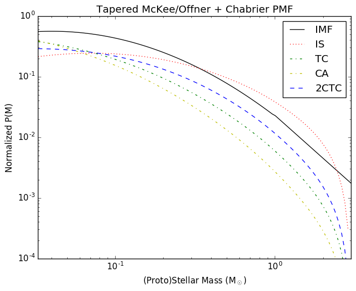
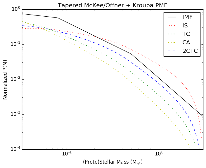
The above plots are the same as before, but with tapered accretion following the prescription in McKee and Offner. The tapering function is apparently arbitrary, and picked purely to enforce smoothness (i.e., prevent a possibly nonphysical instantaneous shutoff of accretion).
Extending to higher masses
When we reevaluate the same functions with mmax=120 instead of 3, we can start to see the high mass end, which is of course power-law dominated. In all cases, the PMF is dominated by the highest-mass sources, since in all cases they take the longest to form.
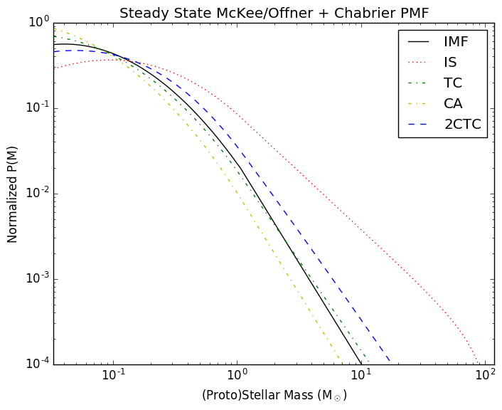
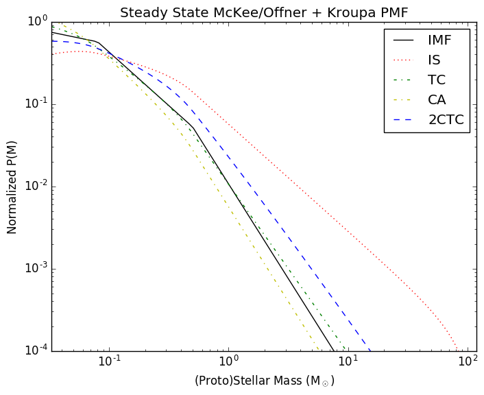
The accretion model changes the slope and the overall ratio of high- to low-mass stars.
These are the mass fractions of various MFs:
- Mass fraction for ChabrierIMF M>10 = 0.192
- Mass fraction for ChabrierPMF_2CTC M>10 = 0.334
- Mass fraction for ChabrierPMF_CA M>10 = 0.150
- Mass fraction for ChabrierPMF_IS M>10 = 0.765
- Mass fraction for ChabrierPMF_TC M>10 = 0.288
- Mass fraction for KroupaIMF M>10 = 0.185
- Mass fraction for KroupaPMF_2CTC M>10 = 0.348
- Mass fraction for KroupaPMF_CA M>10 = 0.148
- Mass fraction for KroupaPMF_IS M>10 = 0.781
- Mass fraction for KroupaPMF_TC M>10 = 0.294
The isothermal sphere case is pretty extremely top-heavy, but all except competitive accretion result in a more top-heavy MF, which is a fairly neat result - it means that simple binning can distinguish between these theories (assuming the parametrization is right). It also means that the SFRs inferred from integrating the high-mass end of the mass function (as I have done in my Sgr B2 paper) is subject to a factor of +/-2x uncertainty depending on the accretion history if we assume steady state.
The next step is to extend this to different accretion histories (tapered, accelerating) and then possibly different star formation histories. I will also create some 'synthetic clusters' using the Robitaille and Zhang models.