\begin{equation*}
P_V(\ln \rho/\rho_0) d \ln \rho = \left[I_1(2\sqrt{\lambda u}) e^{-\lambda-u} \sqrt{\frac{\lambda}{u}} + e^{-\lambda} \delta(u)\right]du
\end{equation*}
\begin{equation*}
P_M(\ln \rho/\rho_0) d \ln \rho = \frac{\rho}{\rho_0} \left[I_1(2\sqrt{\lambda u}) e^{-\lambda-u} \sqrt{\frac{\lambda}{u}} + e^{-\lambda} \delta(u)\right]du
\end{equation*}
\begin{equation*}
u\equiv \frac{\lambda}{1+T} - \frac{\ln \rho/\rho_0}{T} ; (u \geq 0)
\end{equation*}
Moment equations
The important moments are the mean and variance of the volume and mass density
probability distribution and the volume and mass log-density probability
distribution.
The definitions used here are \(E[\rho] \equiv <\rho>_V\), etc. The
variance is computed as \(V[x]=E[x^2]-E[x]^2\), which means we'll need to
compute the moments of various combinations of variables.
Also, \(S_{\ln \rho,V} \equiv V[\ln \rho_V]\)
\begin{equation*}
<\rho>_V \equiv \rho_0 \equiv \int_{-\infty}^{\infty} \rho P_V(\ln \rho/\rho_0) d \ln \rho
\end{equation*}
\begin{equation*}
<\ln \rho>_V \equiv \int_{-\infty}^{\infty} \ln \rho P_V(\ln \rho/\rho_0) d \ln \rho
\end{equation*}
\begin{equation*}
<\rho>_M \equiv \int_{-\infty}^{\infty} \rho (\rho P_V(\ln \rho/\rho_0)) d \ln \rho
\end{equation*}
\begin{equation*}
<\ln \rho>_M \equiv \int_{-\infty}^{\infty} \ln \rho (\rho P_V(\ln \rho/\rho_0)) d \ln \rho
\end{equation*}
\begin{equation*}
<\rho^3>_V \equiv \int_{-\infty}^{\infty} \rho^3 P_V(\ln \rho/\rho_0) d \ln \rho
\end{equation*}
\begin{equation*}
<\ln^2 \rho>_V \equiv \int_{-\infty}^{\infty} (\ln \rho)^2 P_V(\ln \rho/\rho_0)d \ln \rho
\end{equation*}
\begin{equation*}
<\ln^2 \rho>_M \equiv \int_{-\infty}^{\infty} (\ln \rho)^2 \rho P_V(\ln \rho/\rho_0)d \ln \rho
\end{equation*}
In the moment equations, only the input to the PDF is scaled by a mean density
\(\rho_0\); the "weighting factors" for the expectation value are not
(i.e., we are measuring \(E[\rho]\), not \(E[\rho/rho_0]\)).
Delta terms
These can be integrated analytically. In this section, I am just computing the
means; the variances are more complicated.
\begin{equation*}
<\rho>_V \equiv \rho_0 \equiv \int_{-\infty}^{\infty} \rho e^{-\lambda} \delta(\frac{\lambda}{1+T} - \frac{\ln\rho/\rho_0}{T}) \frac{d \ln \rho}{T}
\end{equation*}
\begin{equation*}
<\ln \rho>_V \equiv \int_{-\infty}^{\infty} \ln \rho e^{-\lambda} \delta(\frac{\lambda}{1+T} - \frac{\ln\rho/\rho_0}{T}) \frac{d \ln \rho}{T}
\end{equation*}
\begin{equation*}
<\rho>_M \equiv \int_{-\infty}^{\infty} \rho (\frac{\rho}{\rho_0} e^{-\lambda} \delta(\frac{\lambda}{1+T} - \frac{\ln\rho/\rho_0}{T})) \frac{d \ln \rho}{T}
\end{equation*}
\begin{equation*}
<\ln \rho>_M \equiv \int_{-\infty}^{\infty} \ln \rho (\frac{\rho}{\rho_0} e^{-\lambda} \delta(\frac{\lambda}{1+T} - \frac{\ln\rho/\rho_0}{T})) \frac{d \ln \rho}{T}
\end{equation*}
Substitution: \(v=\frac{\ln \rho/\rho_0}{T}\),
\(dv = \frac{1}{T} d \ln \rho\), \(\rho=\rho_0 e^{v*T}\), \(\ln \rho = v T + \ln \rho_0\)
\begin{equation*}
<\rho>_{V\delta} \equiv \rho_0 \equiv \int_{-\infty}^{\infty} \rho_0 e^{vT} e^{-\lambda} \delta(\frac{\lambda}{1+T} - v) d v
\end{equation*}
\begin{equation*}
<\ln \rho>_{V\delta} \equiv \int_{-\infty}^{\infty} (vT + \ln \rho_0) e^{-\lambda} \delta(\frac{\lambda}{1+T} - v) d v
\end{equation*}
\begin{equation*}
<\rho>_{M\delta} \equiv \int_{-\infty}^{\infty} \rho_0 e^{2vT} ( e^{-\lambda} \delta(\frac{\lambda}{1+T} - v)) d v
\end{equation*}
\begin{equation*}
<\ln \rho>_{M\delta} \equiv \int_{-\infty}^{\infty} (vT + \ln \rho_0) e^{vT} ( e^{-\lambda} \delta(\frac{\lambda}{1+T} - v)) d v
\end{equation*}
Solutions:
\begin{equation*}
<\rho>_{V\delta} = \rho_0 \exp\left[\frac{T \lambda }{1+T} - \lambda\right] = \rho_0 \exp\left[-\lambda \frac{1}{1+T}\right]
\end{equation*}
\begin{equation*}
<\ln \rho>_{V\delta} = e^{-\lambda} \frac{\lambda T}{1+T} + e^{-\lambda} \ln \rho_0
\end{equation*}
\begin{equation*}
<\rho>_{M\delta} = \rho_0 \exp\left[\frac{2 T \lambda }{1+T} - \lambda\right] = \rho_0 \exp\left[\lambda\frac{T-1}{T+1}\right]
\end{equation*}
\begin{equation*}
<\ln \rho>_{M\delta} = \left( \frac{\lambda T}{1+T} + \ln \rho_0 \right) \exp\left[\frac{T \lambda }{1+T} - \lambda\right]
\end{equation*}
\begin{equation*}
= \left( \frac{\lambda T}{1+T} + \ln \rho_0 \right) \exp\left[\frac{ -\lambda }{T+1}\right]
\end{equation*}
(for these next 3, I skipped intermediate steps)
\begin{equation*}
<\rho^3>_{V\delta} = \rho_0^2 \exp\left[\frac{3 T \lambda }{1+T} - \lambda\right] = \rho_0^2 \exp\left[\lambda\frac{2T-1}{T+1}\right]
\end{equation*}
\begin{equation*}
<\ln^2 \rho>_{M\delta} = \left( \frac{\lambda T}{1+T} + \ln \rho_0 \right)^2 \exp\left[\frac{ -\lambda }{T+1}\right]
\end{equation*}
\begin{equation*}
<\ln^2 \rho>_{V\delta} = \left( \frac{\lambda T}{1+T} + \ln \rho_0 \right)^2 e^{-\lambda}
\end{equation*}
Using \(\rho_0=1\) as defined in Hopkins 2013 simplifies all of these a great deal.
PDF Integrals
These cannot be integrated analytically.
However, we can work from a few simple mathematica/sympy results:
\begin{equation*}
\int_0^\infty I_1(x) e^{-x^2/(4L)} dx = e^L - 1
\end{equation*}
\begin{equation*}
\int_0^\infty x^2 I_1(x) e^{-x^2/(4L)} dx = 4 L^2 * e^L
\end{equation*}
\begin{equation*}
\int_0^\infty x^4 I_1(x) e^{-x^2/(4L)} dx = 16 L^3 (L+2) * e^L
\end{equation*}
We use \(L\) instead of \(\lambda\) in these equations because it is often substituted in later equations.
Expectation Value of the Volume-Weighted Density \(E[\rho]\)
\begin{equation*}
E[\rho] \equiv \int \rho P_v(\ln \rho/\rho_0) d \ln \rho = \int \rho \left[I_1(2\sqrt{\lambda u}) e^{-\lambda-u} \sqrt{\frac{\lambda}{u}} + e^{-\lambda} \delta(u)\right]du
\end{equation*}
To get to the form of the above equations, we use the substitution
\begin{equation*}
x = 2\sqrt{\lambda u}
\end{equation*}
which gives us \(\rho\) in terms of \(x\):
\begin{equation*}
\rho = \rho_0 \exp\left[T\left(-\frac{x^2}{4\lambda} + \frac{\lambda}{1+T}\right)\right]
\end{equation*}
and leads to the rearrangement:
\begin{equation*}
E[\rho] = \int \rho_0 \exp\left[T\left(-\frac{x^2}{4\lambda} + \frac{\lambda}{1+T}\right)\right] \left[I_1(x) e^{-x^2/(4\lambda)-\lambda} \right]dx + \rho_0 \exp\left(- \frac{\lambda}{1+T}\right)
\end{equation*}
where the rightmost term is kept from the first moment above. The integral
term can straightforwardly be broken apart into equations of the form shown
above.
\begin{equation*}
L \rightarrow \frac{\lambda}{1+T}
\end{equation*}
\begin{equation*}
E[\rho] = \rho_0 \left[ \exp \left(-\lambda+\frac{T\lambda}{1+T}\right) \int \left[I_1(x) e^{-x^2/(4L)} \right]dx +\exp\left(- \frac{\lambda}{1+T}\right) \right]
\end{equation*}
\begin{equation*}
= \rho_0 \left[ \exp \left(-\lambda+\frac{T\lambda}{1+T}\right)(e^L-1) +\exp\left(- \frac{\lambda}{1+T}\right) \right]
\end{equation*}
\begin{equation*}
= \rho_0 \left[ \exp \left(-\lambda+\frac{T\lambda}{1+T}\right)(e^{\lambda/1+T}-1) +\exp\left(- \frac{\lambda}{1+T}\right) \right]
\end{equation*}
\begin{equation*}
= \rho_0 \left[ e^{-\lambda/(1+T)}(e^{\lambda/1+T}-1) +\exp\left(- \frac{\lambda}{1+T}\right) \right]
\end{equation*}
\begin{equation*}
= \rho_0
\end{equation*}
The same general approach can be followed for all expectation values, but we'll skip the detailed algebra.
Variance of the Volume-Weighted Density \(V[\rho]=S_{\ln \rho,V}\)
\begin{equation*}
V[\rho] = E[\rho^2] - E[\rho]^2 = \rho_0^2 \left[ \exp\left(\lambda\frac{2 T^2}{1+3T+2T^2}\right) - 1 \right]
\end{equation*}
However, the "correction factor" is still important:
\begin{equation*}
V_\delta[\rho] = \rho_0^2 \left[ \exp\left(\lambda\frac{T-1}{T+1}\right) - \exp\left(-2\frac{\lambda}{1+T}\right) \right]
\end{equation*}
Expectation Value of the Mass-Weighted Density \(E_M[\rho]\)
Start from halfway through \(E[\rho]\), simply adding a factor of 2 in the exponent:
\begin{equation*}
E_M[\rho] = \int \rho_0 \exp\left[2T\left(-\frac{x^2}{4\lambda} + \frac{\lambda}{1+T}\right)\right] \left[I_1(x) e^{-x^2/(4\lambda)-\lambda} \right]dx + \rho_0 \exp\left(- \frac{\lambda(T-1)}{1+T}\right)
\end{equation*}
Follow the same math, with \(L=\frac{\lambda}{1+2T}\)
\begin{equation*}
= \rho_0 \left[ \exp \left(-\lambda+\frac{2T\lambda}{1+T}\right)(e^L-1) +\exp\left(- \frac{\lambda(T-1)}{1+T}\right) \right]
\end{equation*}
\begin{equation*}
= \rho_0 \left[ \exp \left(\frac{(T-1)\lambda}{1+T}\right)(e^{\lambda/(1+2T)}-1) +\exp\left(- \frac{\lambda}{1+T}\right) \right]
\end{equation*}
\begin{equation*}
E_M[\rho] = \rho_0 \left[ \exp\left(\lambda\frac{2 T^2}{1+3T+2T^2}\right) - \exp\left(\lambda\frac{T-1}{T+1}\right) + \exp\left(\lambda\frac{T-1}{T+1}\right) \right]
\end{equation*}
The right 2 terms cancel, yielding the value shown in Equation 7 of Hopkins 2013
scaled by \(\rho_0^2\). However, the right-most term is the
correction factor from the Dirac Delta term needed to correct any
numerical computation of the mass-weighted density.
\begin{equation*}
E_{\delta,M}[\rho] = \exp\left(\lambda\frac{T-1}{T+1}\right)
\end{equation*}
\begin{equation*}
E_M[\rho] = \rho_0 \exp\left(\lambda\frac{2 T^2}{1+3T+2T^2}\right)
\end{equation*}
Expectation Value of the Mass-Weighted Density Squared \(E_M[\rho^2]\)
\begin{equation*}
E_M[\rho^2] = \int \rho^2 \frac{\rho}{\rho_0} e^{-\lambda} \left[I_1(x) e^{-x^2/(4\lambda)} \right]dx + \int \rho^2 \frac{\rho}{\rho_0} e^{-\lambda} \delta(u) du
\end{equation*}
\begin{equation*}
E_{\delta,M}[\rho^2] = \rho_0^2 \exp\left[\lambda\frac{2T-1}{T+1}\right]
\end{equation*}
\begin{equation*}
E_{left}[\rho^2] = e^{-\lambda} \int
\rho_0^2 \exp\left[3T\left(-\frac{x^2}{4\lambda} + \frac{\lambda}{1+T}\right)\right]
\left[I_1(x) e^{-x^2/(4\lambda)} \right]
dx
\end{equation*}
\begin{equation*}
= \rho_0^2 \exp\left[\frac{(2T-1)\lambda}{1+T}\right]
\int I_1(x) e^{-(3T+1)x^2/(4\lambda)} dx
\end{equation*}
\begin{equation*}
= \rho_0^2 \exp\left[\frac{(2T-1)\lambda}{1+T}\right]
\left( \exp\left[\frac{\lambda}{3T+1}\right] - 1\right)
\end{equation*}
\begin{equation*}
= \rho_0^2 \left(\exp\left[\frac{6\lambda T^2}{3T^2+4T+1}\right] - \exp\left[\frac{(2T-1)\lambda}{1+T}\right] \right)
\end{equation*}
\begin{equation*}
E_{M}[\rho^2] = \rho_0^2 \exp\left[\frac{6\lambda T^2}{3T^2+4T+1}\right]
\end{equation*}
Variance of the Mass-Weighted Density \(V_M[\rho] = E_M[\rho^2] - E_M[\rho]^2\)
Since correction factors are given for \(E_M[\rho^2]\) and
\(E_M[\rho]\), they are not included separately here:
\begin{equation*}
V_M[\rho] = E_M[\rho^2] - E_M[\rho]^2
= \rho_0^2 \left( \exp\left[\frac{6\lambda T^2}{3T^2+4T+1}\right]
-\exp\left[\lambda\frac{4 T^2}{1+3T+2T^2}\right]
\right)
\end{equation*}
Expectation Value of the Volume-Weighted Log Density \(E[\ln \rho]\)
\begin{equation*}
E[\ln \rho] = \int \ln \rho e^{-\lambda} \left[I_1(x) e^{-x^2/(4\lambda)} \right]dx + \int \ln \rho e^{-\lambda} \delta(u) du
\end{equation*}
\begin{equation*}
E_\delta[\ln \rho] = e^{-\lambda} \left[ \frac{\lambda T}{1+T} + \ln \rho_0 \right]
\end{equation*}
\begin{equation*}
E_{left}[\ln \rho] = \int \left[\ln \rho_0 + T\left(-\frac{x^2}{4\lambda} + \frac{\lambda}{1+T}\right) \right] e^{-\lambda} \left[I_1(x) e^{-x^2/(4\lambda)} \right]dx
\end{equation*}
\begin{equation*}
= e^{-\lambda} \left( \int \left[\ln \rho_0 + \frac{T\lambda}{1+T}\right] \left[I_1(x) e^{-x^2/(4\lambda)} \right]dx
- \int \frac{T x^2}{4\lambda} \left[I_1(x) e^{-x^2/(4\lambda)} \right]dx \right)
\end{equation*}
\begin{equation*}
= e^{-\lambda} \left( \int \left[\ln \rho_0 + \frac{T\lambda}{1+T}\right](e^{\lambda}-1)
- \frac{4 T \lambda^2 e^{\lambda}}{4\lambda} \right)
\end{equation*}
\begin{equation*}
= \left( \left[\ln \rho_0 + \frac{T\lambda}{1+T}\right](1-e^{-\lambda})
- T \lambda \right)
\end{equation*}
\begin{equation*}
E[\ln \rho] = \ln \rho_0 + \frac{T\lambda}{1+T} - T \lambda
\end{equation*}
\begin{equation*}
= \ln \rho_0 - \frac{T^2\lambda}{1+T}
\end{equation*}
Expectation Value of the Mass-Weighted Log Density \(E_M[\ln \rho]\)
\begin{equation*}
E_M[\ln \rho] = \int \ln \rho \frac{\rho}{\rho_0} e^{-\lambda} \left[I_1(x) e^{-x^2/(4\lambda)} \right]dx + \int \ln \rho \frac{\rho}{\rho_0} e^{-\lambda} \delta(u) du
\end{equation*}
\begin{equation*}
E_\delta[\ln \rho] = \left( \frac{\lambda T}{1+T} + \ln \rho_0 \right) \exp\left[\frac{ -\lambda }{T+1}\right]
\end{equation*}
\begin{equation*}
E_{left}[\ln \rho] = e^{-\lambda} \int \left[
\left(\ln \rho_0 + T\left(-\frac{x^2}{4\lambda} + \frac{\lambda}{1+T}\right) \right)
\exp\left(T\left(-\frac{x^2}{4\lambda} + \frac{\lambda}{1+T}\right)\right) \right]
\left[I_1(x) e^{-x^2/(4\lambda)} \right]dx
\end{equation*}
Again, separate into integrable terms:
\begin{equation*}
= \exp\left(\frac{T\lambda}{1+T} -\lambda\right) \left[
\left(\ln \rho_0 + \frac{T\lambda}{1+T} \right) \left[I_1(x) e^{-(1+T)x^2/(4\lambda)} \right] +
\left(-\frac{Tx^2}{4\lambda} \right) \left[I_1(x) e^{-(1+T)x^2/(4\lambda)} \right]
\right]
\end{equation*}
\begin{equation*}
L = \frac{\lambda}{1+T}
\end{equation*}
\begin{equation*}
E_{left}[\ln \rho] = \exp\left(\frac{T\lambda}{1+T} -\lambda\right) \left[
\left(\ln \rho_0 + \frac{T\lambda}{1+T} \right) \left(\exp\left[\frac{\lambda}{1+T}\right]-1\right) +
\left(-\frac{T}{4\lambda} \right) \left(\frac{4 \lambda^2}{(1+T)^2} \exp\left[\frac{\lambda}{1+T}\right]\right)
\right]
\end{equation*}
\begin{equation*}
E_{left}[\ln \rho] = \exp\left(\frac{-\lambda}{1+T}\right) \left[
\left(\ln \rho_0 + \frac{T\lambda}{1+T} \right) \left(\exp\left[\frac{\lambda}{1+T}\right]-1\right) +
\left(-\frac{T}{4\lambda} \right) \left(\frac{4 \lambda^2}{(1+T)^2} \exp\left[\frac{\lambda}{1+T}\right]\right)
\right]
\end{equation*}
\begin{equation*}
E_{left}[\ln \rho] =
\left(\ln \rho_0 + \frac{T\lambda}{1+T} \right) \left(1-\exp\left[\frac{-\lambda}{1+T}\right]\right) -
\left(\frac{ T \lambda}{(1+T)^2} \right)
\end{equation*}
\begin{equation*}
E_M[\ln \rho] = \left(\ln \rho_0 + \frac{T\lambda}{1+T} \right) -
\left(\frac{ T \lambda}{(1+T)^2} \right)
\end{equation*}
\begin{equation*}
= \ln \rho_0 + \frac{T^2\lambda}{(1+T)^2}
\end{equation*}
Expectation Value of the Mass-Weighted Log Density Squared \(E_M[\ln^2 \rho]\)
\begin{equation*}
E_M[\ln^2 \rho] = \int (\ln \rho)^2 \frac{\rho}{\rho_0} e^{-\lambda} \left[I_1(x) e^{-x^2/(4\lambda)} \right]dx + \int (\ln \rho)^2 \frac{\rho}{\rho_0} e^{-\lambda} \delta(u) du
\end{equation*}
\begin{equation*}
E_\delta[\ln^2 \rho] = \left( \frac{\lambda T}{1+T} + \ln \rho_0 \right)^2 \exp\left[\frac{ -\lambda }{T+1}\right]
\end{equation*}
\begin{equation*}
E_{left}[\ln^2 \rho] = e^{-\lambda} \int \left[
\left(\ln \rho_0 + T\left(-\frac{x^2}{4\lambda} + \frac{\lambda}{1+T}\right) \right)^2
\exp\left(T\left(-\frac{x^2}{4\lambda} + \frac{\lambda}{1+T}\right)\right) \right]
\left[I_1(x) e^{-x^2/(4\lambda)} \right]dx
\end{equation*}
This time it's just too ugly. Define a new variable:
\begin{equation*}
Q = \ln \rho_0 + \frac{T\lambda}{1+T}
\end{equation*}
\begin{equation*}
E_{left}[\ln^2 \rho] = e^{-\lambda/(1+T)} \int \left[
\left(Q -\frac{T x^2}{4\lambda} \right)^2
\exp\left(-\frac{Tx^2}{4\lambda} \right) \right]
\left[I_1(x) e^{-x^2/(4\lambda)} \right]dx
\end{equation*}
\begin{equation*}
E_{left}[\ln^2 \rho] = e^{-\lambda/(1+T)} \int \left[
\left(Q^2 - 2 Q \frac{T x^2}{4\lambda} + \frac{T^2 x^4}{16\lambda^2} \right)
\left[I_1(x) e^{-(1+T)x^2/(4\lambda)} \right]
\right]dx
\end{equation*}
\begin{equation*}
E_{left}[\ln^2 \rho] = e^{-\lambda/(1+T)} \left[
Q^2 (e^{\lambda/(1+T)}-1)
- 2 Q \frac{T}{4\lambda} \left(\frac{4\lambda^2}{(1+T)^2} e^{\lambda/(1+T)}\right)
+ \frac{T^2}{16\lambda^2} \left(16 \frac{\lambda^3}{(1+T)^3} (\frac{\lambda}{1+T}+2) e^{\lambda/(1+T)} \right)
\right]
\end{equation*}
\begin{equation*}
E_{left}[\ln^2 \rho] =
Q^2 (1-e^{-\lambda/(1+T)})
- 2 Q \frac{T\lambda}{(1+T)^2}
+ \frac{\lambda T^2}{(1+T)^3} \left(\frac{\lambda}{1+T}+2\right)
\end{equation*}
Add back the \(\delta\) termG
\begin{equation*}
E_M[\ln^2 \rho] =
Q^2
- 2 Q \frac{T\lambda}{(1+T)^2}
+ \frac{\lambda T^2}{(1+T)^3} \left(\frac{\lambda}{1+T}+2\right)
\end{equation*}
Re-expand to see if it's simplifiable....
\begin{equation*}
E_M[\ln^2 \rho] =
\left(\ln \rho_0 + \frac{T\lambda}{1+T}\right)^2
- 2 \left(\ln \rho_0 + \frac{T\lambda}{1+T}\right) \frac{T\lambda}{(1+T)^2}
+ \frac{\lambda T^2}{(1+T)^3} \left(\frac{\lambda}{1+T}+2\right)
\end{equation*}
\begin{equation*}
E_M[\ln^2 \rho] =
\ln^2 \rho_0 + 2 \ln \rho_0 \frac{T\lambda}{1+T} + \frac{T^2\lambda^2}{(1+T)^2}
- 2 \ln \rho_0 \frac{T\lambda}{(1+T)^2} - 2 \frac{T\lambda}{1+T} \frac{T\lambda}{(1+T)^2}
+ 2 \frac{\lambda T^2}{(1+T)^3}
+ \frac{\lambda T^2}{(1+T)^3} \frac{\lambda}{1+T}
\end{equation*}
\begin{equation*}
E_M[\ln^2 \rho] =
\ln^2 \rho_0 + 2 \ln \rho_0 \left(\frac{T\lambda}{1+T} - \frac{T\lambda}{(1+T)^2}\right)
+ \frac{T^2\lambda^2(1+T)}{(1+T)^3}
- 2 \frac{T^2\lambda^2}{(1+T)^3}
+ 2 \frac{\lambda T^2}{(1+T)^3}
+ \frac{\lambda^2 T^2}{(1+T)^4}
\end{equation*}
\begin{equation*}
E_M[\ln^2 \rho] =
\ln^2 \rho_0 + 2 \ln \rho_0 \left(\frac{T^2\lambda}{1+T}\right)
+ \frac{T^2\lambda^2(1+T)}{(1+T)^3}
- 2 \frac{T^2\lambda^2}{(1+T)^3}
+ 2 \frac{\lambda T^2}{(1+T)^3}
+ \frac{\lambda^2 T^2}{(1+T)^4}
\end{equation*}
\begin{equation*}
= \ln^2 \rho_0 + 2 \ln \rho_0 \frac{T^2 \lambda}{(1+T)^2}
+ \left(\frac{\lambda T^2}{(1+T)^2}\right)^2
+ \frac{2\lambda T^2}{(1+T)^3}
\end{equation*}
\begin{equation*}
= \left(\ln \rho_0 + \frac{T^2\lambda}{(1+T)^2}\right)^2 +
\frac{2\lambda T^2}{(1+T)^3}
\end{equation*}
As expected, we recover the correct relation from Hopkins 2013:
\begin{equation*}
S_{\ln \rho,M} = E_M[\ln \rho^2] - E_M[\ln \rho]^2 =
\ln^2 \rho_0 + 2 \ln \rho_0 \frac{T^2 \lambda}{(1+T)^2}
+ \left(\frac{\lambda T^2}{(1+T)^2}\right)^2 + \frac{2\lambda T^2}{(1+T)^3}
- \left(\ln \rho_0 + \frac{T^2\lambda}{(1+T)^2}\right)^2
\end{equation*}
\begin{equation*}
= \frac{2\lambda T^2}{(1+T)^3}
\end{equation*}
independent of \(\rho_0\).
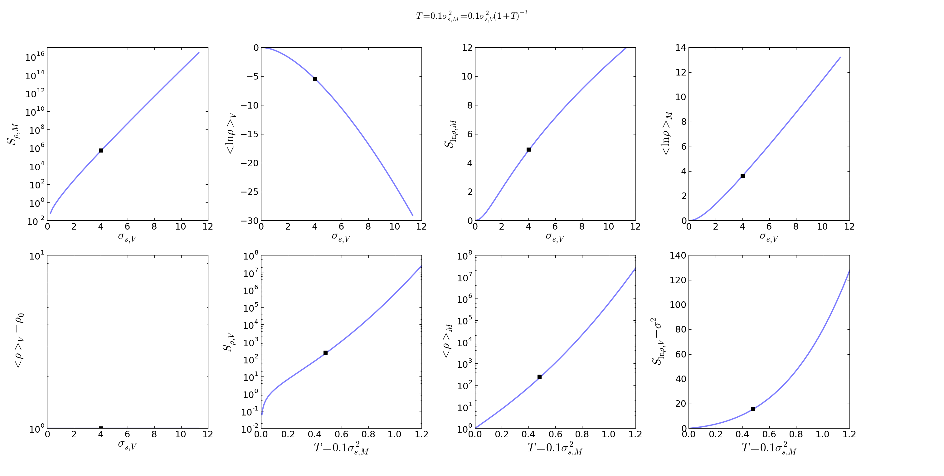
Properties of the Hopkins PDF
I began this investigation in order to find out whether a different parameter,
i.e. something related to the compressiveness of the turbulent driving, could
be responsible for the "discrepancy" between the Formaldehyde-derived density
and the volume-averaged density of some clouds.
I naively expected that, in compressive turbulence, more of the mass will be
concentrated at higher density, which should drive up the mass-weighted mean
density.
Hopkins 2013 showed that \(T\sim\mathcal{M}_C\). If this is taken on
face value, without recognizing the relation between \(T\) and
\(\sigma\), it means that for fixed \(\sigma\),
\(<\rho>_M\propto e^{-T^2}\).
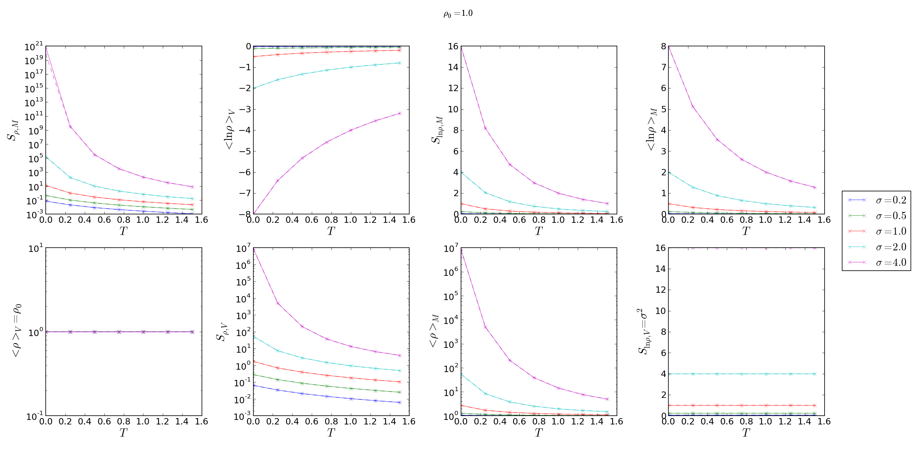
This figure shows the relation of the various moments and \(T\). The plots
show both the "theoretical" result (i.e., doing the integral by hand) and the
numerical result with 50,000 data points plus a correction for the
\(\delta\) terms; the agreement is essentially perfect excepting some
numerical noise (the only visible discrepancy is for a perfect lognormal at
high \(\sigma_V\)):
However, Hopkins 2013 also found that simulations generally produced
\(T\sim0.1\sigma_{s,M}^2\) (though a relation of the form \(T\sim 0.25
\ln(1+0.25\sigma_{s,M}^4)\) is also a good fit).
If you use the simpler of these relations, the expected relationship (mean mass
increasing with increasing "compressiveness") is recovered. However, it comes
with an increasing \(\sigma_s\). In these plots, half are labeled with
\(\sigma\) and the others are labeled with \(T\), though the two are
equivalent. The highest \(\sigma_s\) observed in any of the simulations
shown in Hopkins 2013 was about \(\sigma_s=4\) (marked with a black
square below), so the maximum \(\rho_M/\rho_V \sim 10^2\).