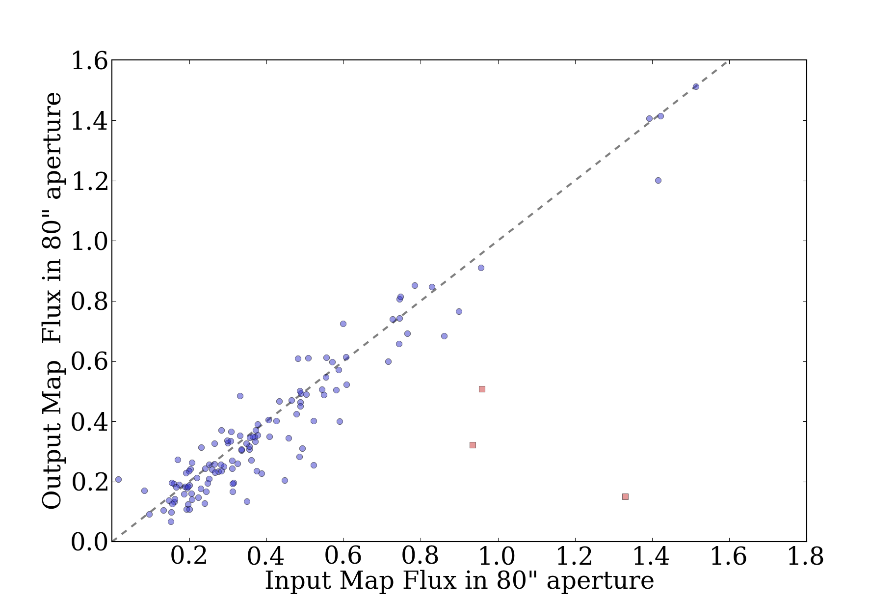
In the last couple drafts of the BGPS paper (e.g. the May 15, 2013 draft), we've included a single simulation demonstrating the flux recovery of the Bolocat:


These figures are regarded as very important, as they demonstrate the capability of recovering accurate flux density measurements from a realistic sky using bolocat.
However, the above figures show a simulation only for one set of parameters, with \(\alpha=1\) in the power-law flux distribution, which unfortunately is not realistic according to "Figure 8":

So I've started up a new experiment, experiment #23, to examine this problem.
The problem has a few layers:
- The reason I used \(\alpha=1\) is that it looks much like a realistic BGPS map after processing, in the sense that most of the field is empty but there are a few hundred sources in the map. However, \(\alpha=1\) is not a realistic representation of the measured power spectra.
- \(\alpha=2\) maps with the previous normalization had a peak value of 18 Jy, which resulted in heavily signal-dominated output maps that did not resemble BGPS maps.
- The normalization is tricky. One of the key goals of the simulations was to test the effect of different atmospheric to astrophysical signal ratios on the angular transfer function; in order to accomplish this, it was necessary to scale the atmospheric power based on the astrophysical power at its peak in fourier space. i.e., in real timestreams, we can measure the astrophysical to atmospheric power ratio, but we have to perform that measurement somewhere that the angular transfer function is known to be reliable. This is done at about 1 Hz.
- The normalization is important because of the noise level. In the simulations, we use a fixed noise level of about 30 mJy in the timestreams to match our best observations (though it is not difficult to scale this to other levels). This fixed noise level means that, for some normalizations, all pixels are statistically significant. Also, even though the noise level is fixed, it will be higher because of intrinsic noise in a power-law distributed map.
- The normalizations used in experiment #21, the angular transfer function measurement, were selected such that there would be high signal-to-noise at all angular scales. This means that white noise would not be dominant on any angular scale, since white noise is equivalent to \(\alpha=0\). So it wasn't crazy to use these ridiculously high-flux maps, but it is not feasible to use the same maps for analysis of point sources. In maps for which we're interested in small-angular-scale features (<100"), we want the maps to be primarily noise-dominated with a handful of bright features either caused by adding point sources directly or from the local peaks in the power-law distributed flux.
Some notes along the way:
- Using a power-law background, the point-source sensitivity is much worse than without a power-law background. This is intuitive: a 100 mJy source on a 200 mJy background (which may easily include power fluctuations on the smallest scales of comparable magnitude) is not going to be recovered.
- Doubly important: a 1 Jy source should have peak amplitude 1 Jy, but the current method of adding point sources adds them as delta functions that are later convolved, conserving the total flux rather than the peak flux. This needs to be changed! (has been now)
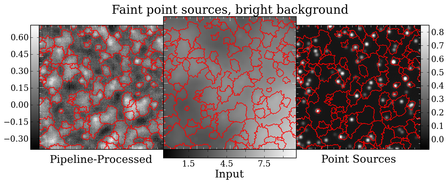
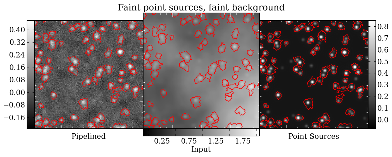
Here are some examples of what the before/after look like with point sources added. The first has bright sources, the second faint sources:
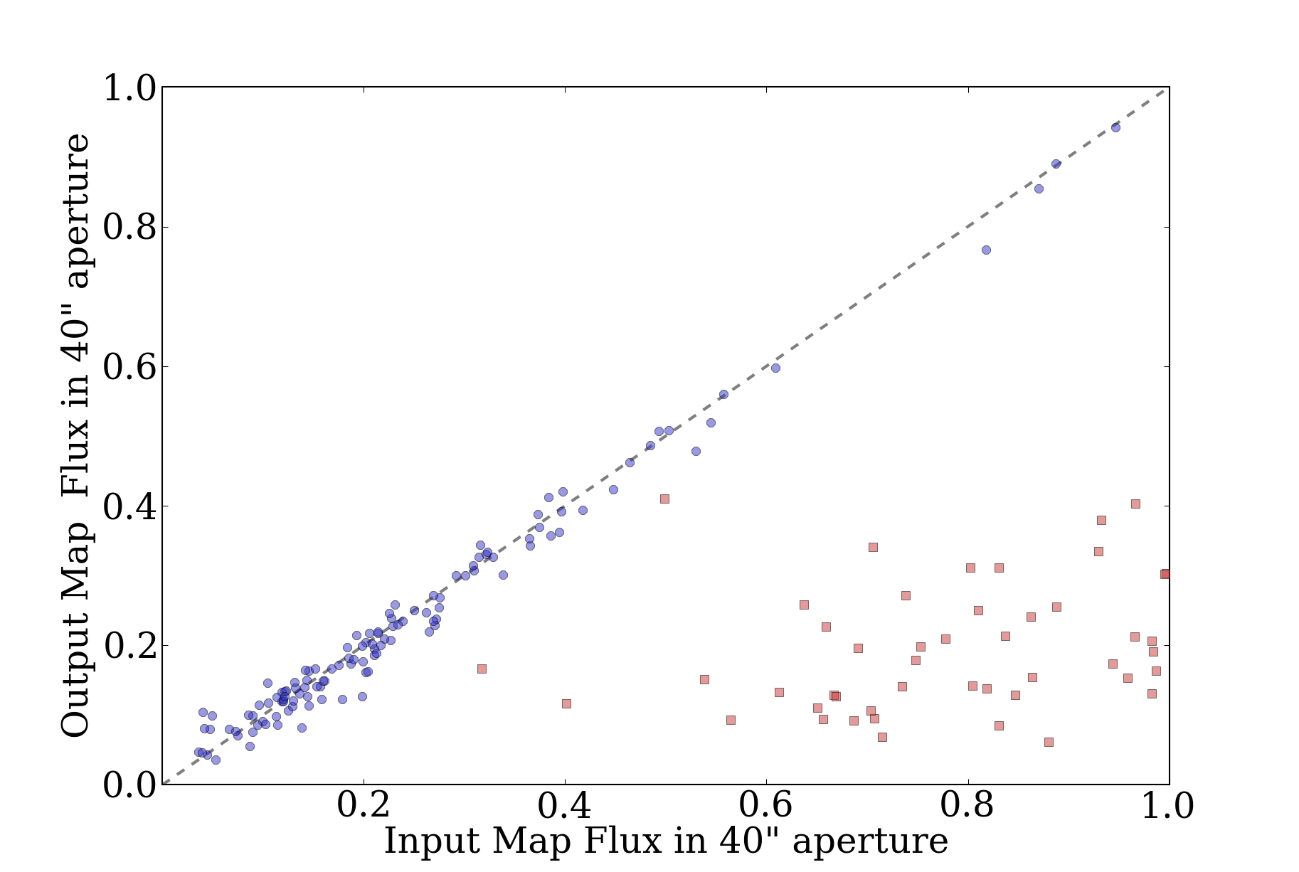
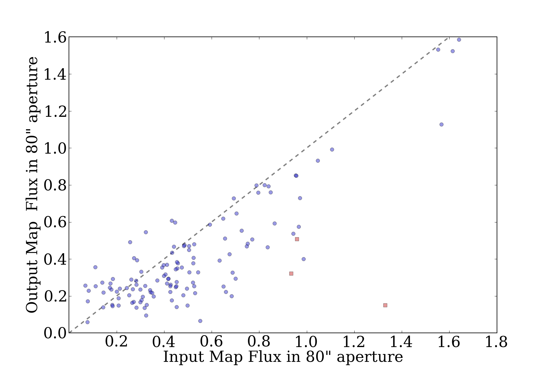
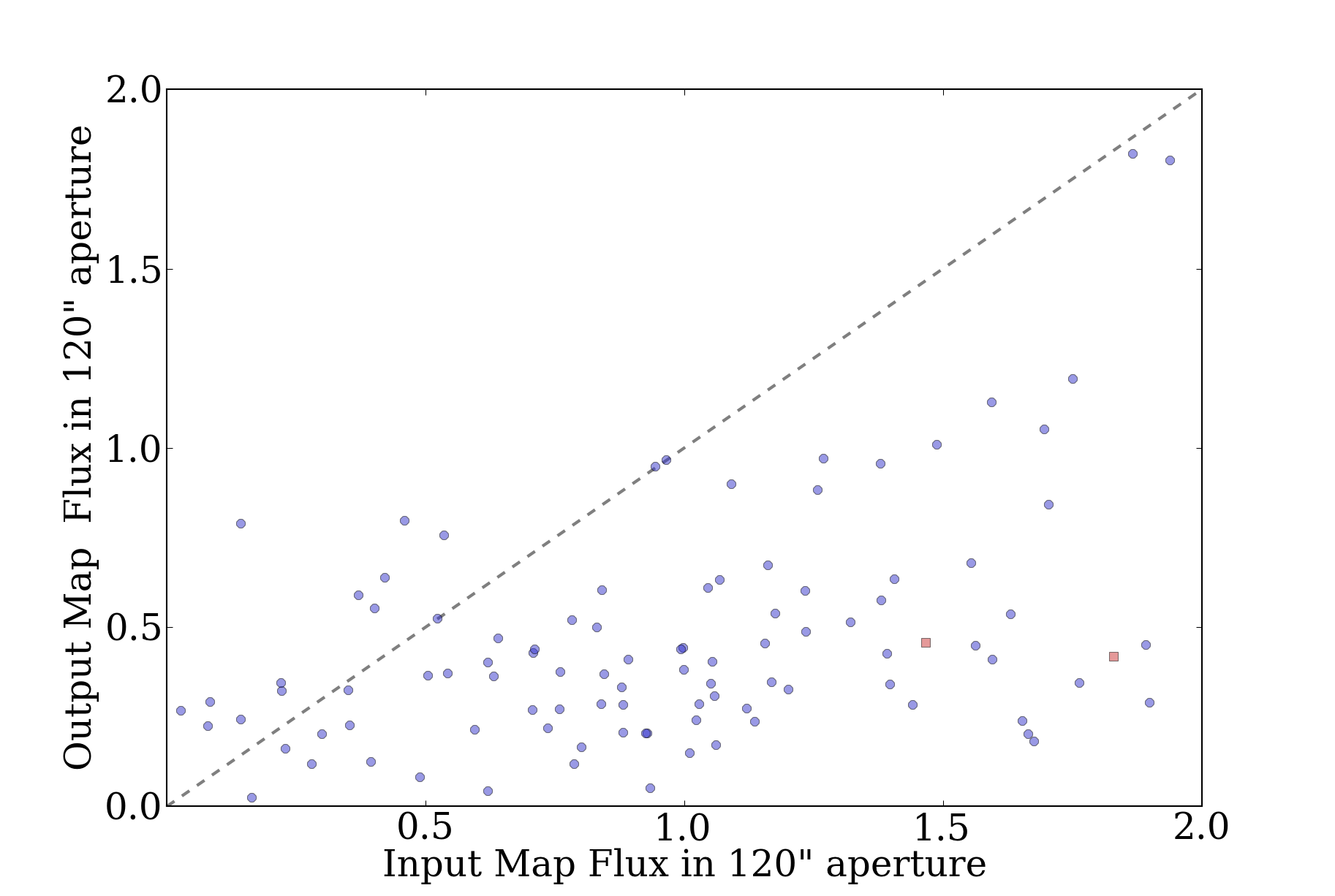
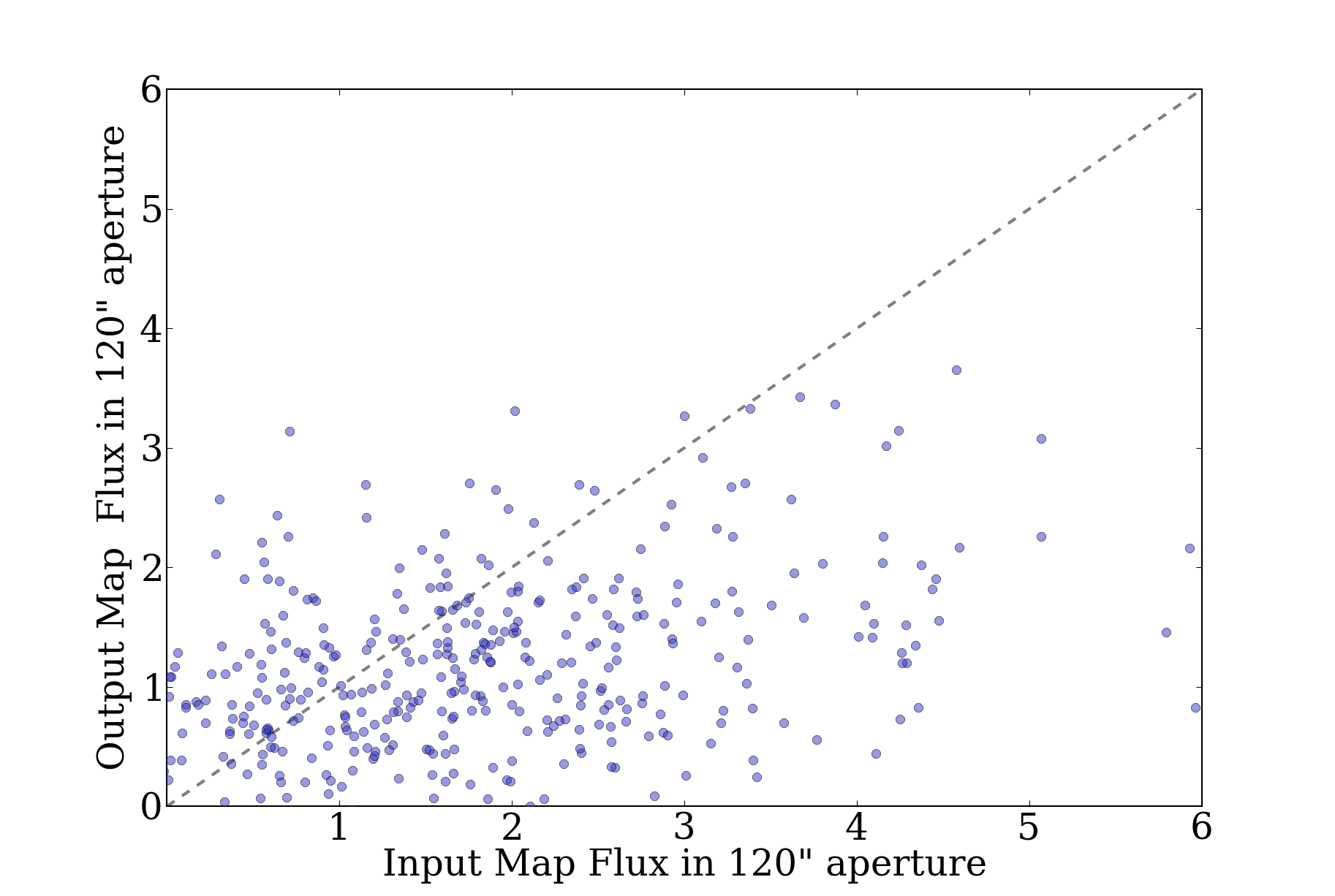
With these new figures, the 40" apertures work fine, but the 120" apertures are still utterly junk. This does not make sense.
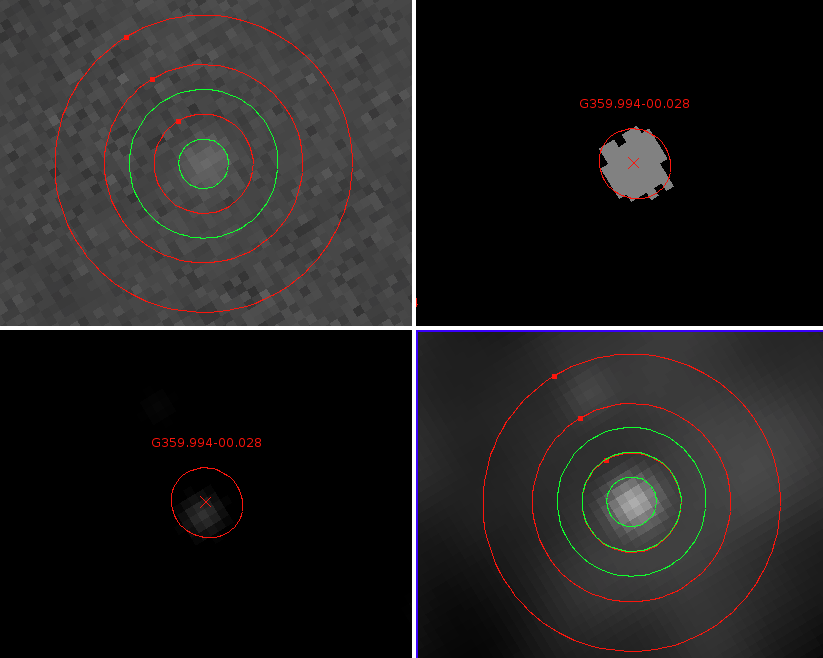
A careful analysis of a single source shows that something is wrong. Here are some annular extractions followed by the image:
Input Map:
reg sum npix    mean    median  min         max     var         stddev      rms
--- --- ----    ----    ------  ---         ---     ---         ------      ---
1   26.3323 22  1.19692 1.18083 1.10787     1.28825 0.00208826  0.0456975   1.1978
2   77.8553 74  1.0521  1.047   1.00426     1.123   0.000929507 0.0304878   1.05254
3   124.868 122 1.02351 1.02869 0.996566    1.04427 0.000260295 0.0161337   1.02363

Output Map:
reg sum         npix    mean        median      min         max         var         stddev      rms
--- ---         ----    ----        ------      ---         ---         ---         ------      ---
1   3.89157     23      0.169199    0.175204    0.086872    0.255151    0.00206254  0.0454152   0.175188
2   2.06843     74      0.0279517   0.0275116   -0.0695484  0.155258    0.00210834  0.0459167   0.0537554
3   0.502601    123     0.00408619  0.00629906  -0.121023   0.0834974   0.00143969  0.0379432   0.0381626

Backgrounds:
Input Map:
reg  sum      npix  mean      median    min       max      var          stddev     rms
---  ---      ----  ----      ------    ---       ---      ---          ------     ---
1    297.054  291   1.0208    1.02293   0.98094   1.05234  0.000313419  0.0177037  1.02096
3    2538.6   2618  0.969671  0.972413  0.859551  1.12495  0.0015557    0.0394423  0.970473

Output Map:
reg  sum      npix  mean        median      min        max       var         stddev     rms
---  ---      ----  ----        ------      ---        ---       ---         ------     ---
1    1.49461  291   0.00513613  0.00729431  -0.121023  0.133141  0.001586    0.0398247  0.0401545
3    5.83372  2618  0.00222831  0.00194597  -0.195075  0.181155  0.00211747  0.046016   0.0460699

Bolocat for this source:
In [200]: fields
Out[200]: ['FLUX_40', 'FLUX_40_NOBG', 'BG_40', 'FLUX_120', 'FLUX_120_NOBG', 'BG_120']

In [198]: [inp[61][f] for f in fields]
Out[198]: [0.1896538, 1.3536235, 0.38071653, 0.83893013, 10.77737, 0.42352486]

In [199]: [m20[61][f] for f in fields]
Out[199]: [0.18015364, 0.18674377, -0.016305592, 0.2868295, 0.29759517, -0.00027596406]
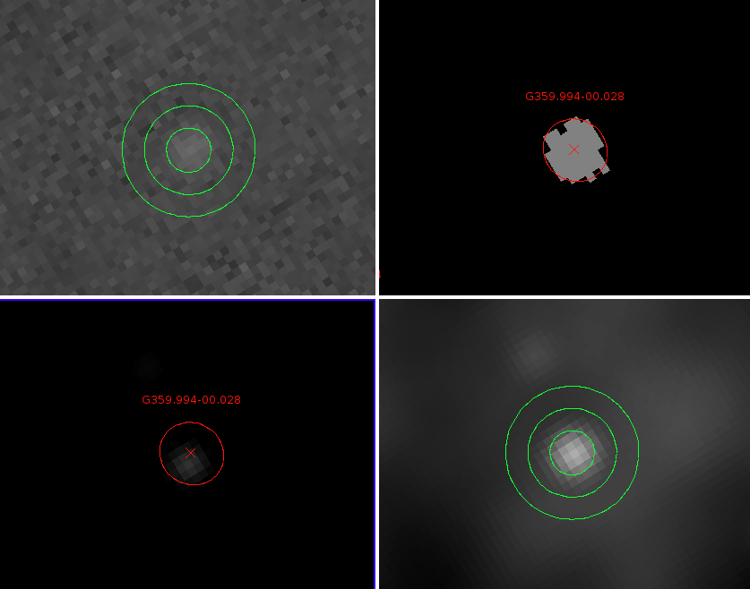
With background apertures:
However, note that the background are computed using the mmm.pro sky-background estimation procedure over a range \(2r\) to \(4r\) (i.e., 40-80" and 120-240" radius for the 40" and 120" diameter apertures).
The numbers shown by ds9 disagree fairly severely with those from bolocat. In particular, it appears that the background estimate returned by mmm.pro is off by a factor of 2, in this case giving 0.42 instead of 0.97. Turns out this was due to an indexing error that did not affect the pipeline results in any way.
Out of date analysis: Bolocat's flux total in the 120" aperture is 10.77 Jy/beam, background is 0.42 Jy/beam. There are 218 pixels. The resulting flux should be (10.77-0.42*218/23.8), but this gives 6.9 instead of the expected 0.84. Why?
If we do the same with the ds9 numbers, we get a total of 9.62 Jy/beam, background 0.97 Jy/beam average, so: (9.62 - 0.97*218/23.8) = 0.74. This is consistent with bolocat, and very very wrong.
If we take our background to be 1.02 instead of 0.97, we get 0.28 Jy/beam, which is exactly the right answer according to the pipeline. 1.02 comes from taking a much more local background subtraction from r=40 to r=80 arcsec, which isn't really acceptable. If we go from r=60 to r=120, the disagreement remains fairly bad, with f=0.38 Jy/beam, but certainly a lot better.
Bolocat after the correction:
In [297]: [m20[61][f] for f in fields]
Out[297]: [0.18015364, 0.18674377, 0.00578439, 0.25477698, 0.29759517, 0.0041758944]

In [298]: [inp[61][f] for f in fields]
Out[298]: [0.1896538, 1.3536235, 1.0216572, 0.40137589, 10.77737, 1.0119308]
This may mean that we'll need to re-do aperture extraction with a tighter background region everywhere. I made the change to object_photometry.
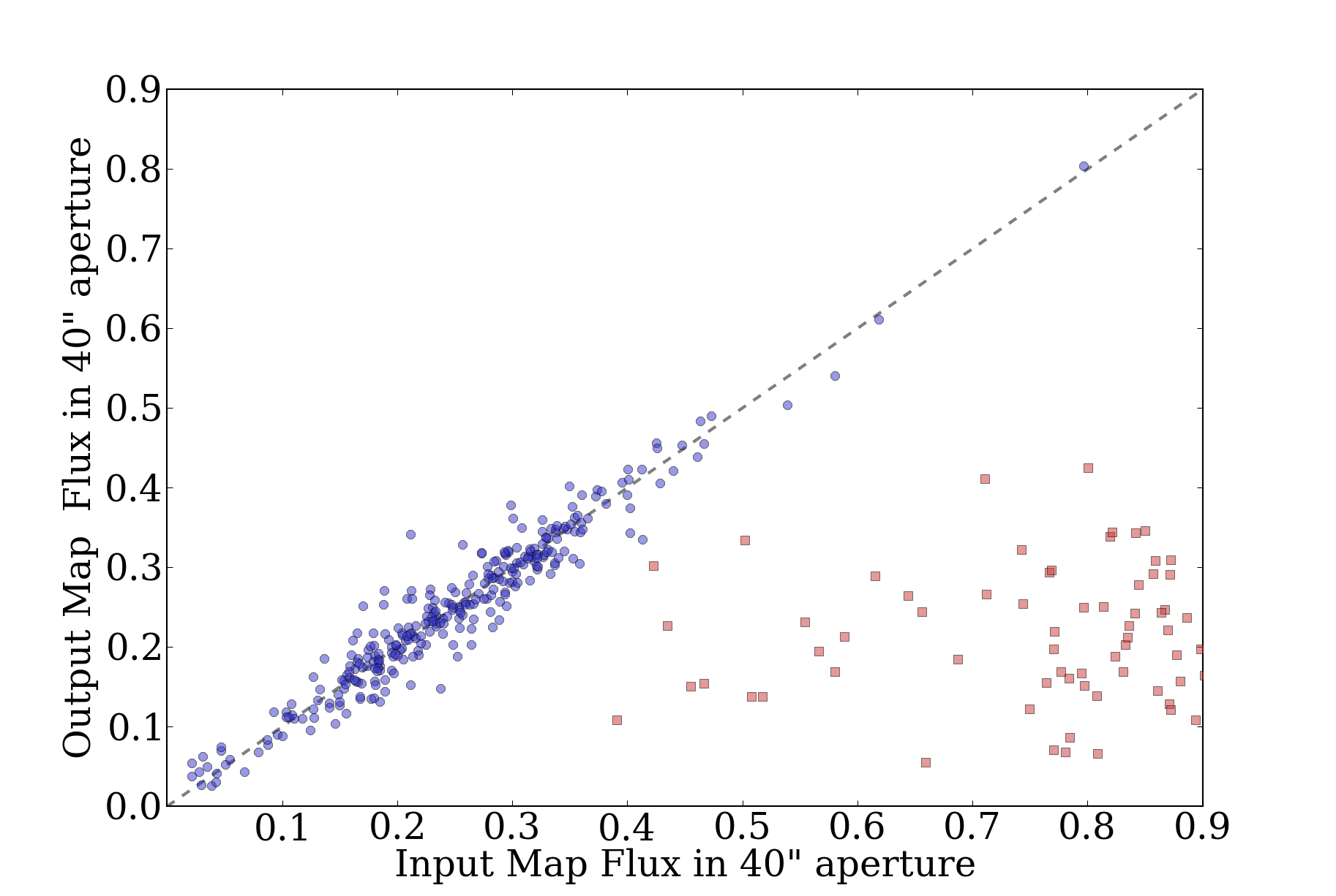
However, even with the change, even in the best case, FLUX_120 appears to be totally unreliable. FLUX_80 is acceptable with the change, but only for bright sources (for faint sources, <1 Jy, there is no recovery at all - I think this must be an issue of the source brightness still not being calculated correctly):
I'll have to continue this analysis tomorrow once the full suite of simulations has completed, but I strongly suspect that we'll have to recommend strictly against using FLUX_120 if the background is expected to be \(\alpha=2\) distributed.
Day 2
The simulations have partly completed. After correcting the error with convolved point sources vs. delta functions, I reset the flux distributions to be 0.05 to 1.0 Jy for the "faint" distribution and 0.1 to 50.0 Jy for the "bright" distribution (both with power-law distributions \(\alpha=2\)).
The results can be summarized:
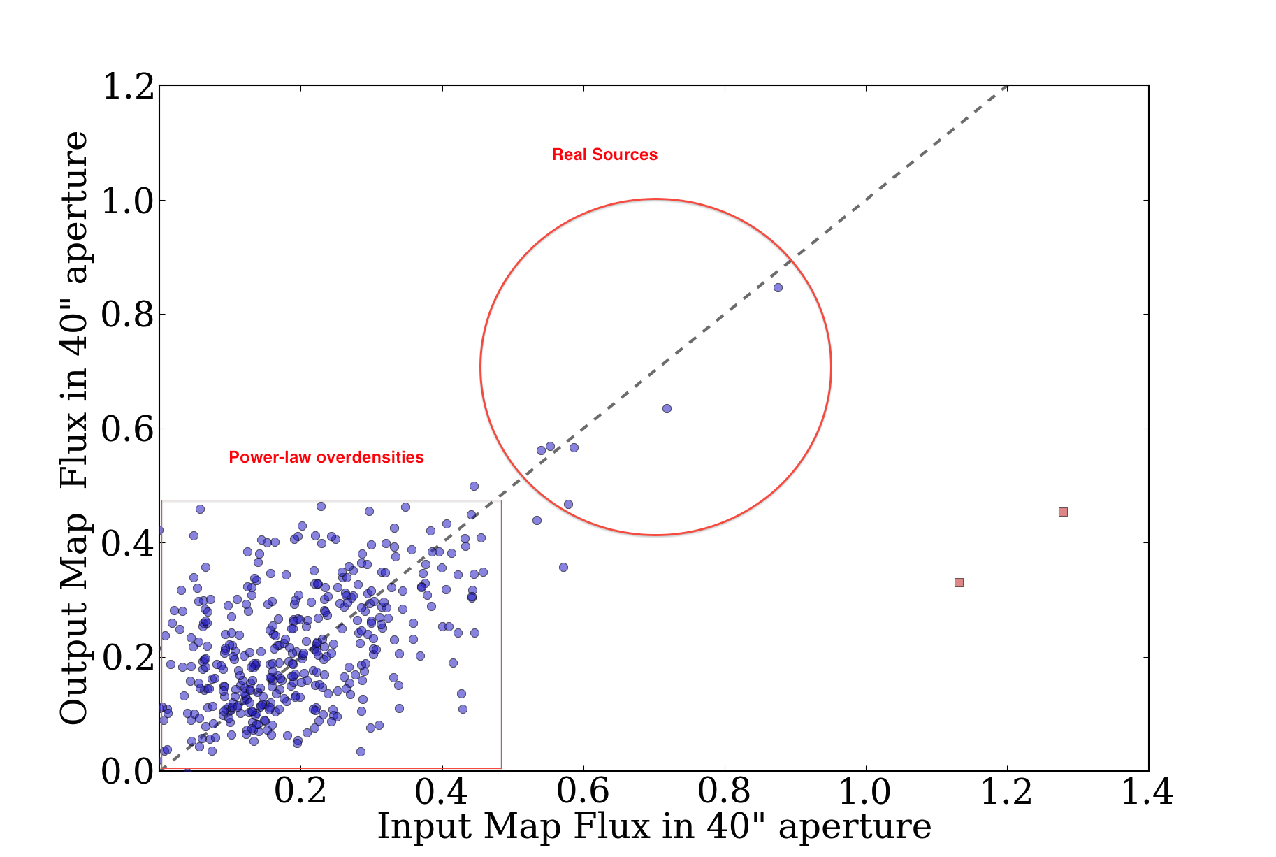
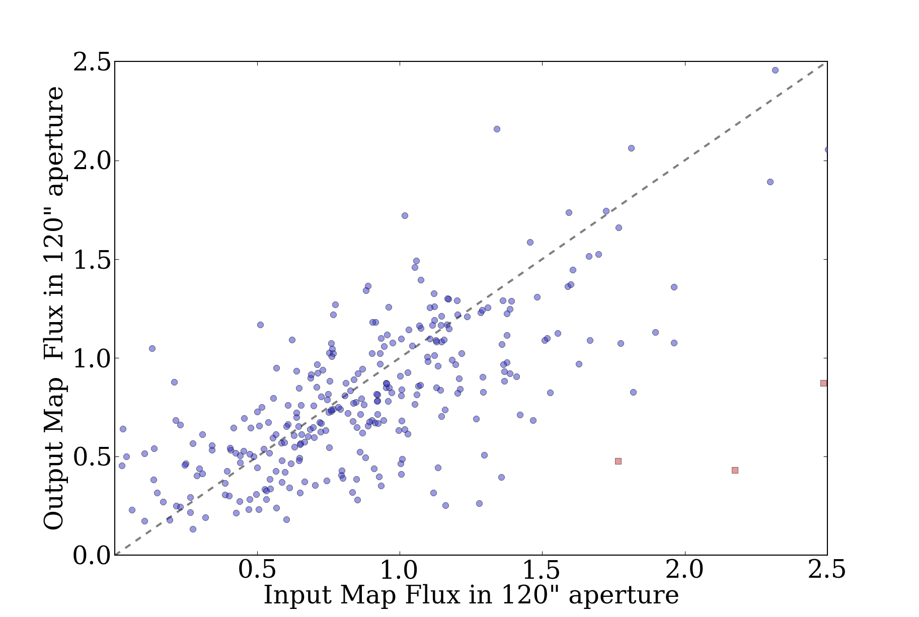
- In the presence of complex background, i.e power-law distributed flux density with amplitude comparable to the detected source brightness, only the smallest aperture (40") is reliable (i.e., recovers a flux in the input and processed map).
- The recovered flux density has a very high dispersion in the presence of high-amplitude power-law flux. "Very high" = \(\sigma \gtrsim 1\) around a mean of 1.
- There is no evident dependence of the maps on the atmospheric properties. Therefore, there's no sense in varying the atmospheric properties in the simulations.
I decided the simulations needed changing again. First, there was excessive sampling in astro/atmo parameter space; this is not needed (see point 3). More important is the power-law distribution map's peak flux. Also, it is more important to get decent sampling of bright-ish sources than to have a "physically accurate" point source distribution; the distribution of sources does not affect the recovery, but it does affect the signal-to-noise of the recovery measurement. Please don't ask me to defend this statement; it would require another 10 hours of computer time + me time that I really don't want to allocate, but I'm confident that it is true.
The essential conclusion is that, for \(\alpha=2\), point source recovery is only possible if the point source is brighter than the background, which is a very intuitive result. Background annulus subtraction isn't very effective at pulling out sources.
Conclusions:
- These experiments show that source recovery is very poor in the presence of a bright power-law background: it is not possible to reliably extract point sources from a map filled with power-law distributed emission brighter than or comparable to the point sources.
- The 120" apertures aren't really good for anything.
- There is so much source-extraction parameter space out there that any further study would really deserve its own paper.
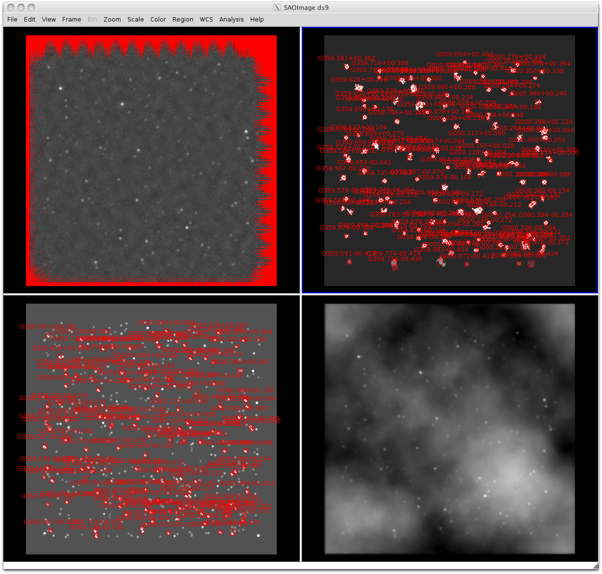
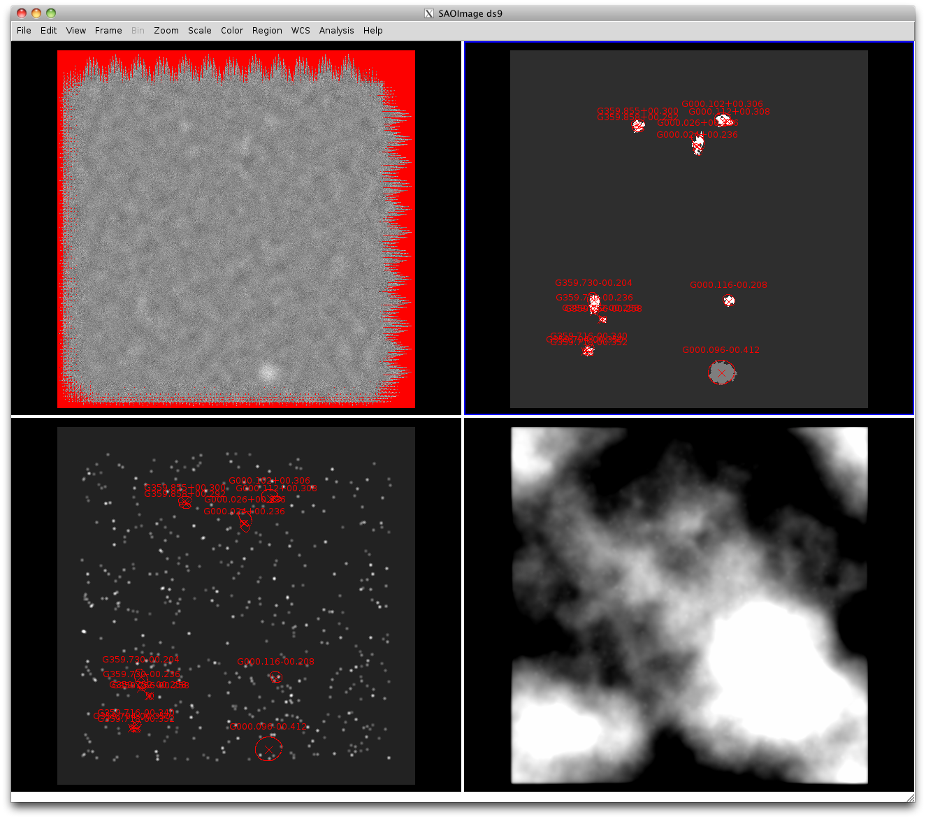
Additional plots of interest:
40" aperture in the presence of a bright background with faint sources:
Versus the same with a faint background:
Compare these to the 120" equivalents (bright then faint background):
It's fairly easy to see why there are issues with the bright background and the 120" apertures. In this image, bright background on the left, faint background on the right, with faint sources (0.1-1 Jy).
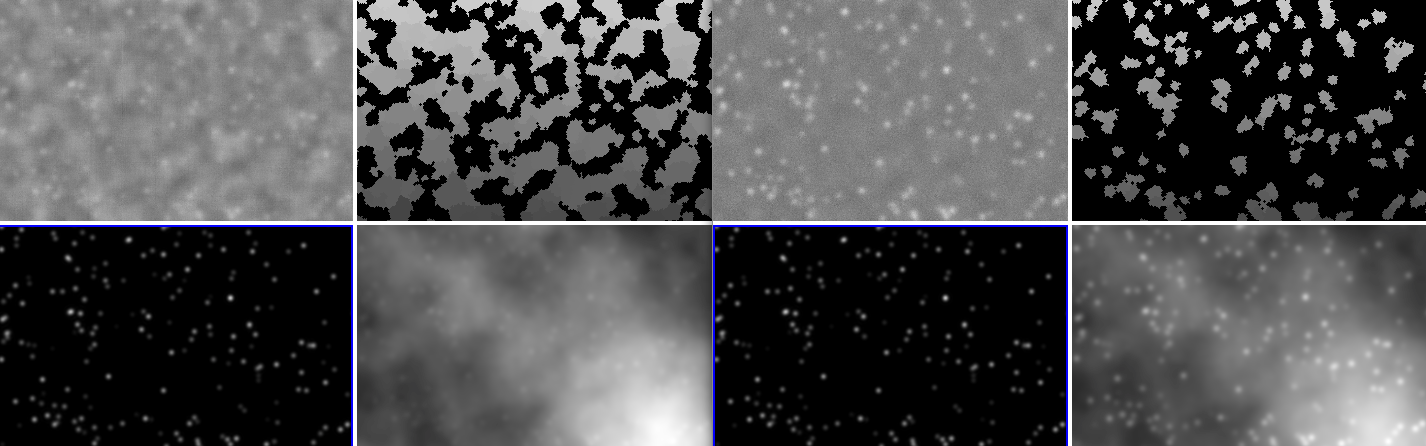
It's more helpful to look at that previous image with the source contours superposed. These images really give a nice feel for what it means to have point sources subsumed in \(\alpha=2\) background.